CS180 Project 3: Image Warping and Mosaicing

Overview

In this project, I implemented an end-to-end mosaicing pipeline. In Part A, the process involved shooting photos from the same center of projection, computing homographies to align them, warping images using both nearest-neighbor and bilinear interpolation, and finally blending them into seamless mosaics.

In Part B, I automated the alignment by first detecting corners with the Harris operator and ANMS, then extracting 40x40 grayscale patches downsamples to 8x8 (bias/gain-normalized), matching features using SSD distances with the Lowe ratio test, then estimating a robust homography with 4-point RANSAC.

A.1: Shoot and Digitize Pictures

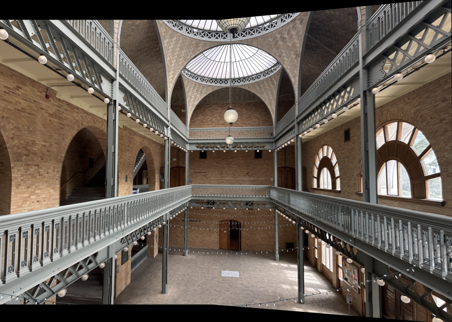
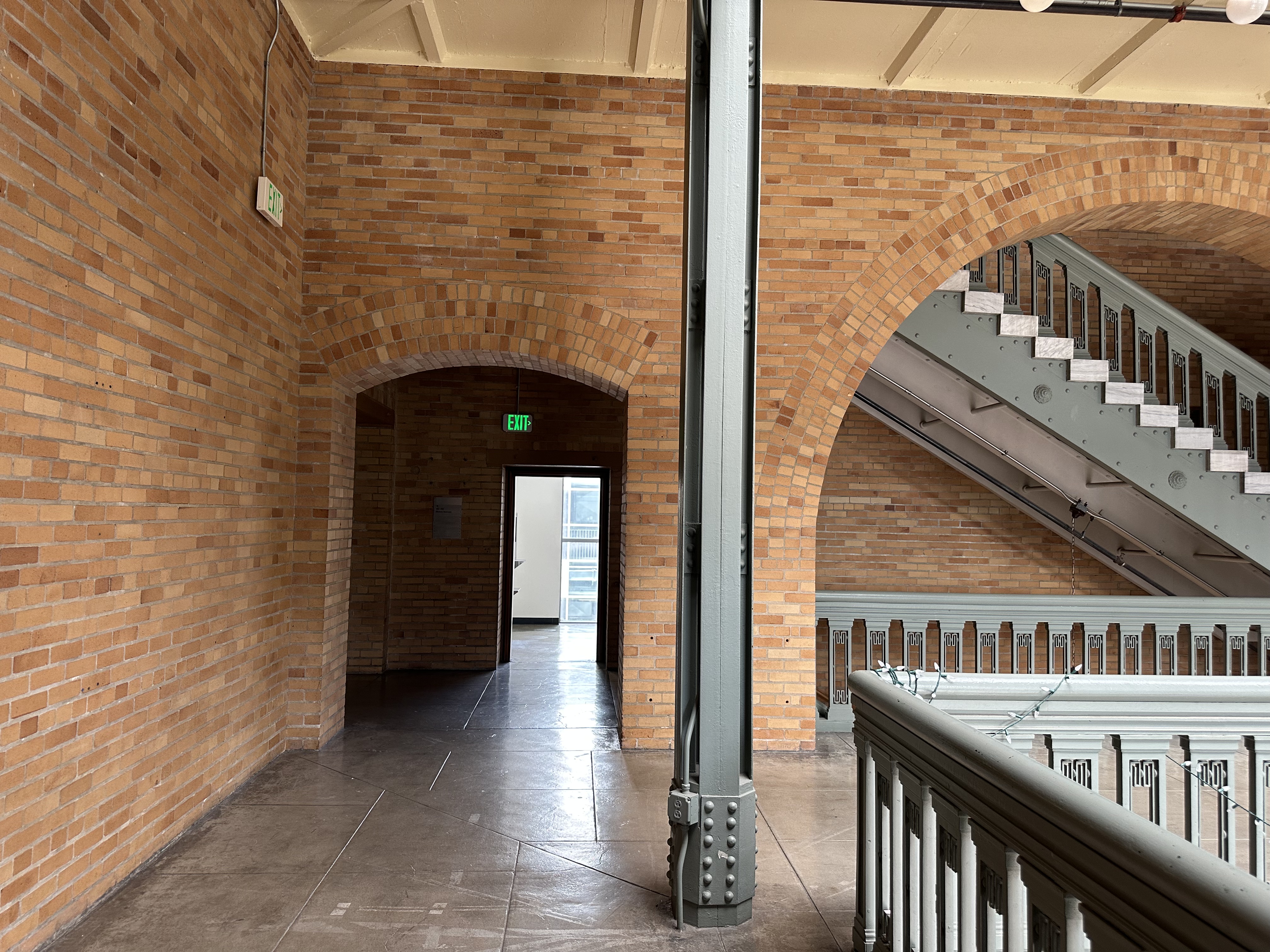
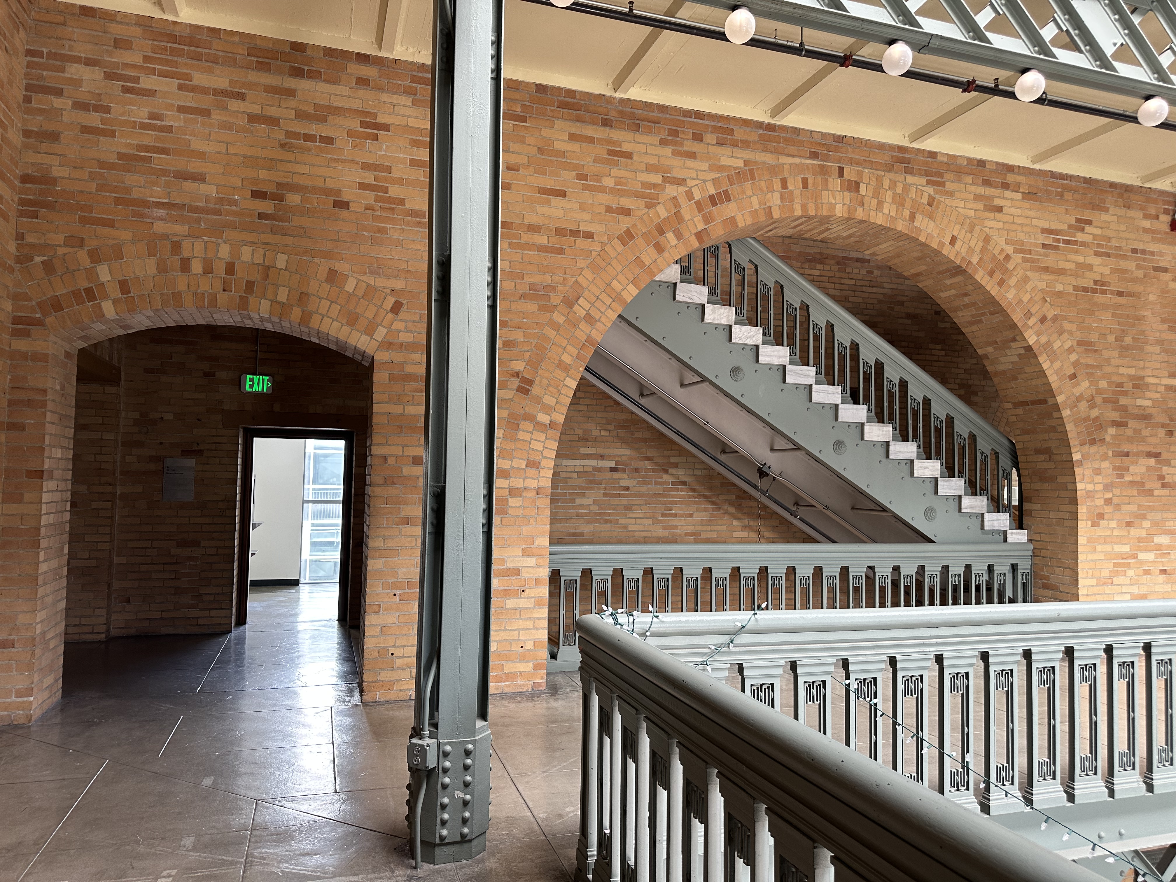
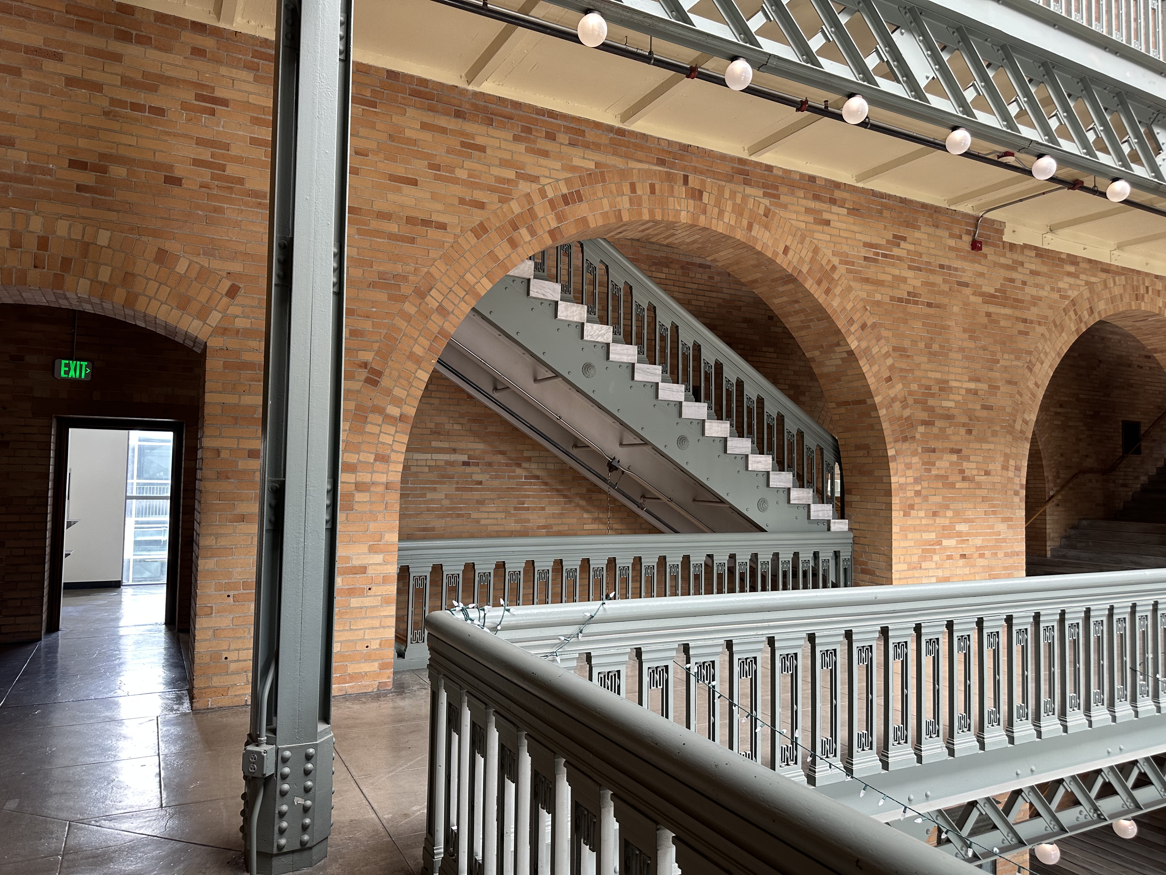
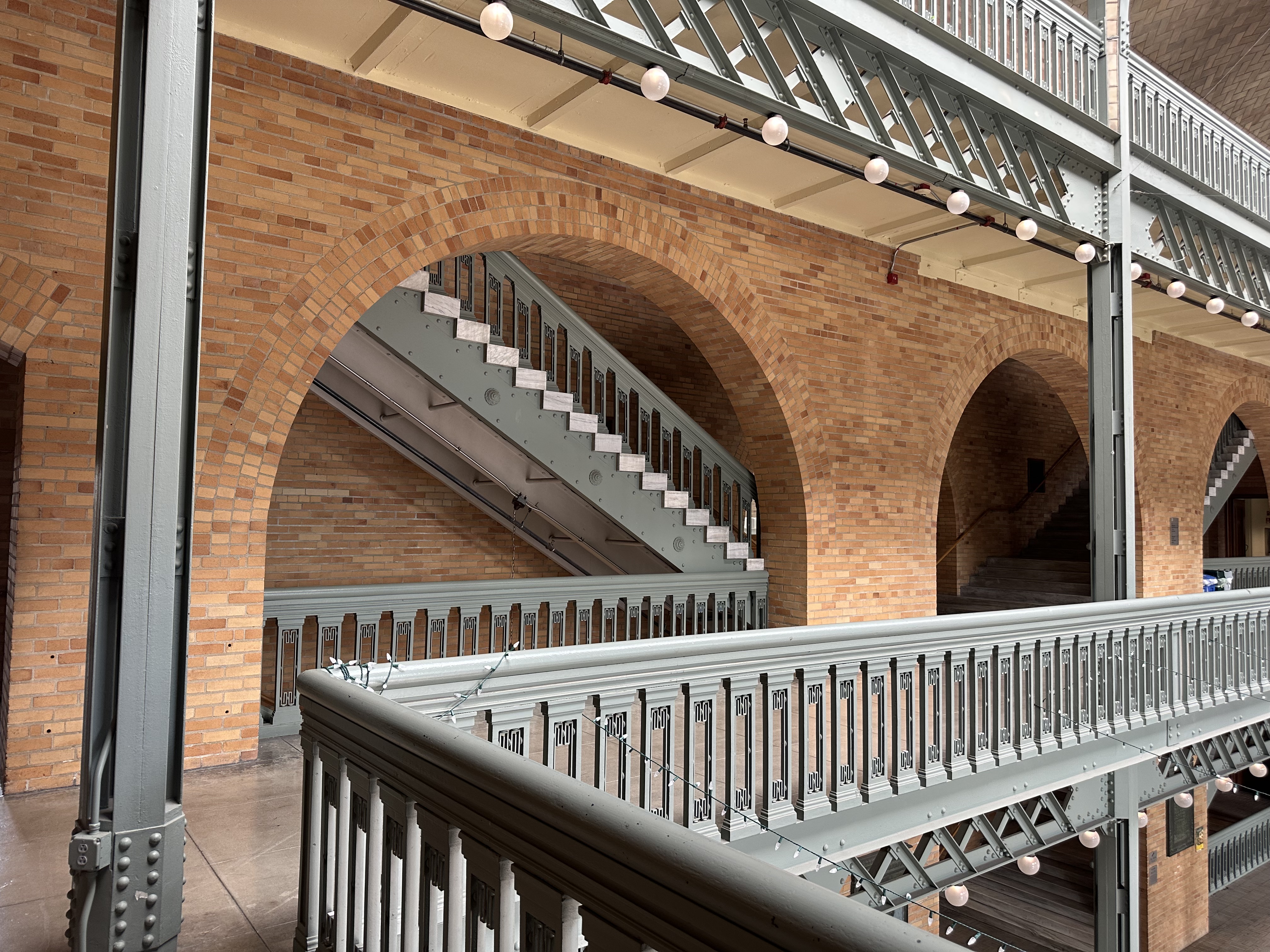
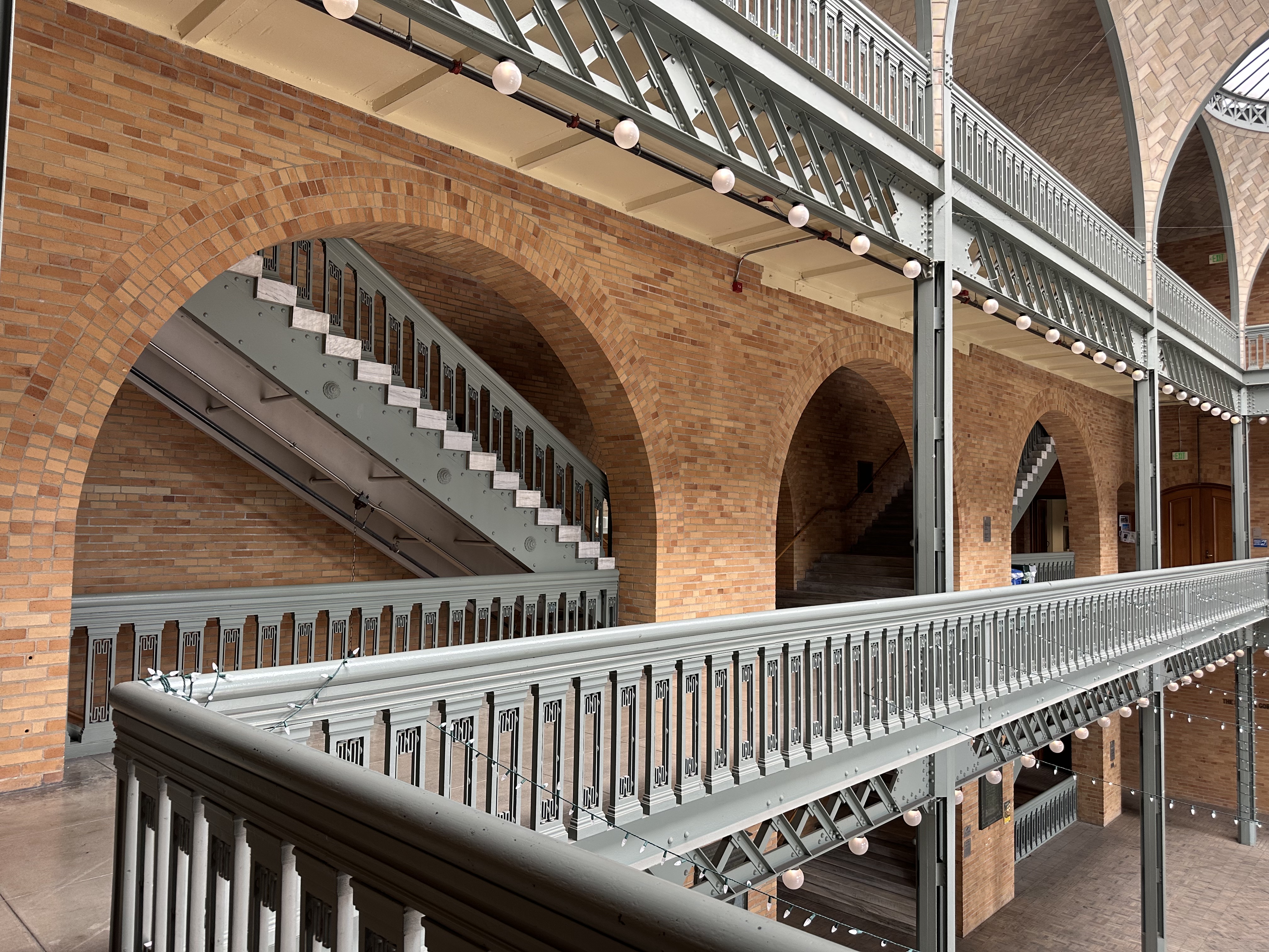
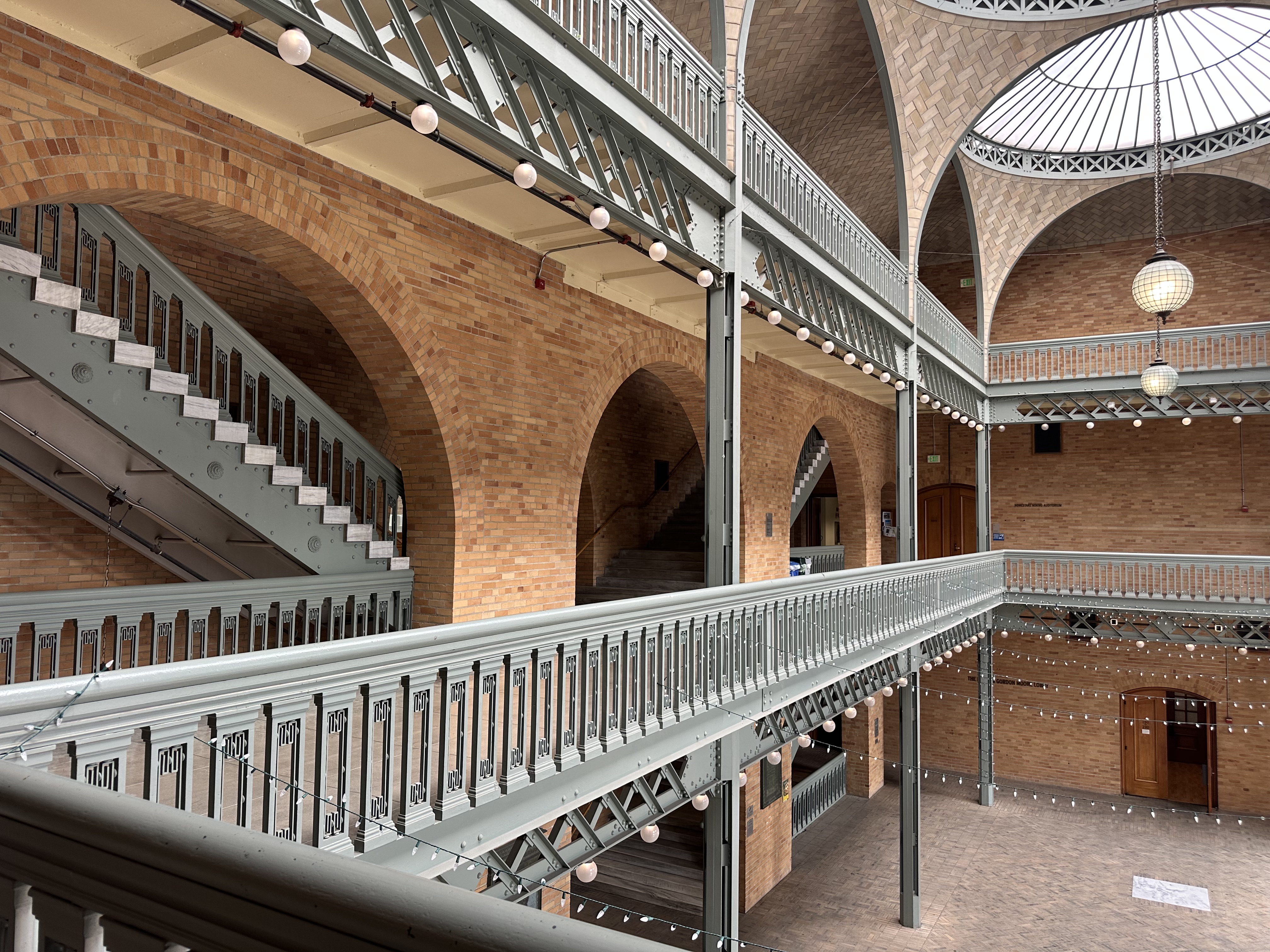
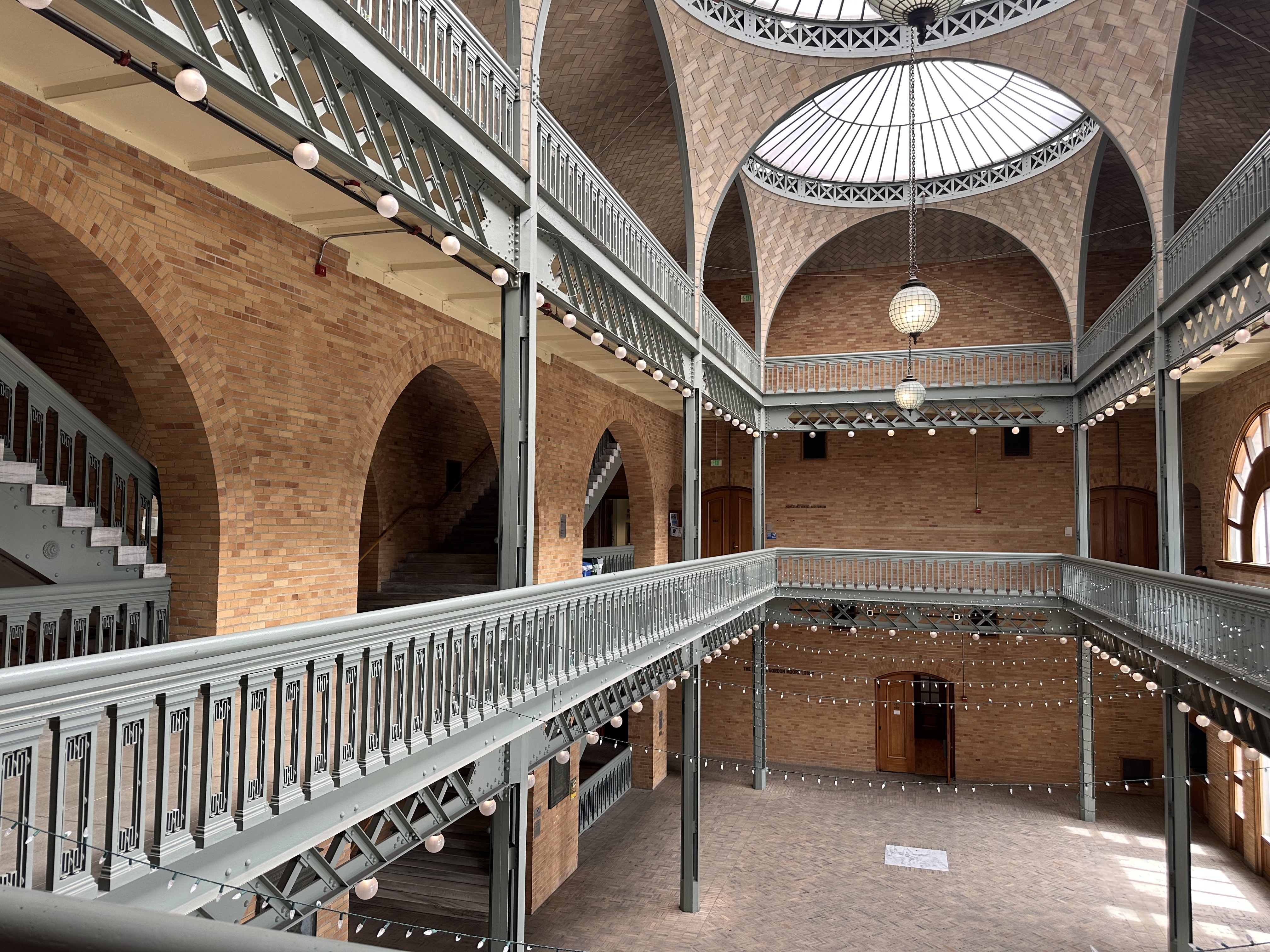
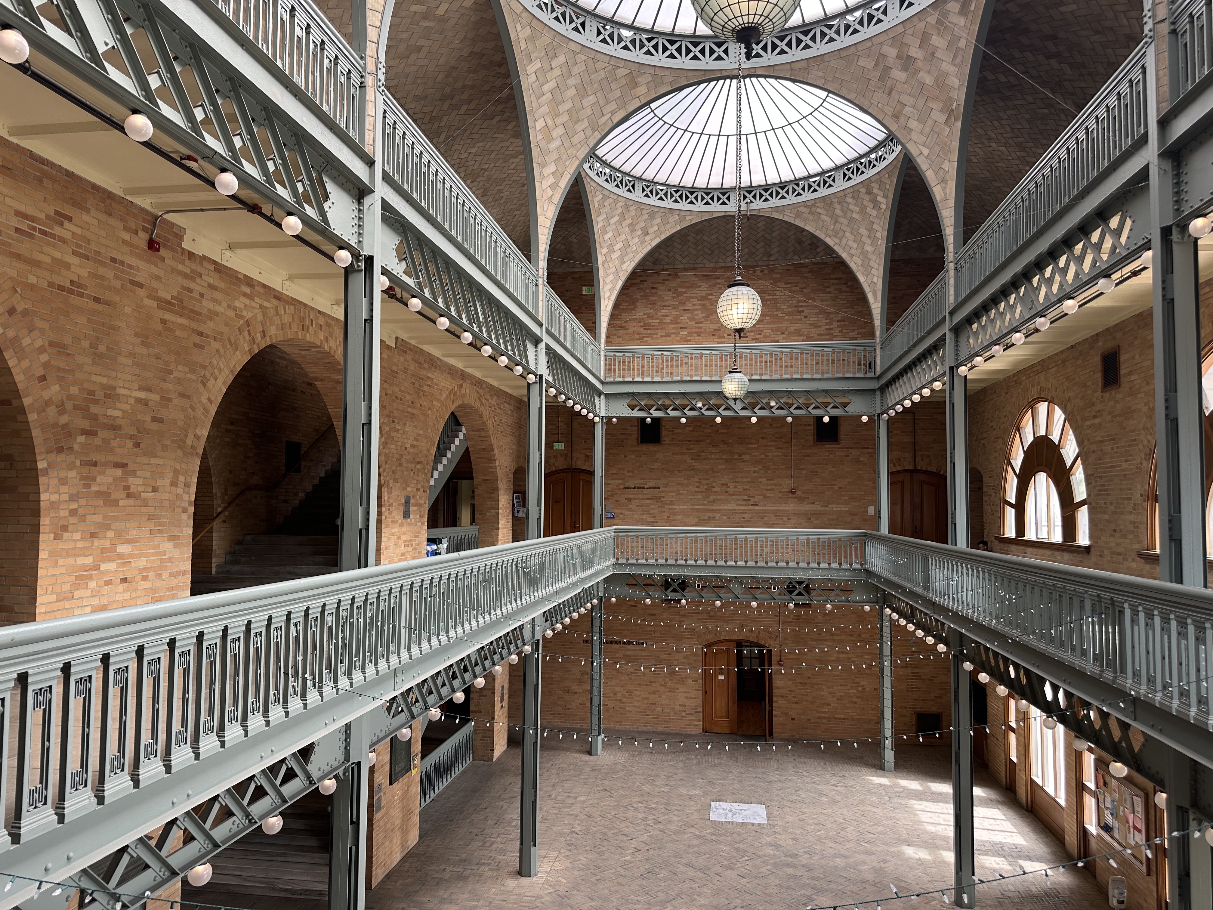
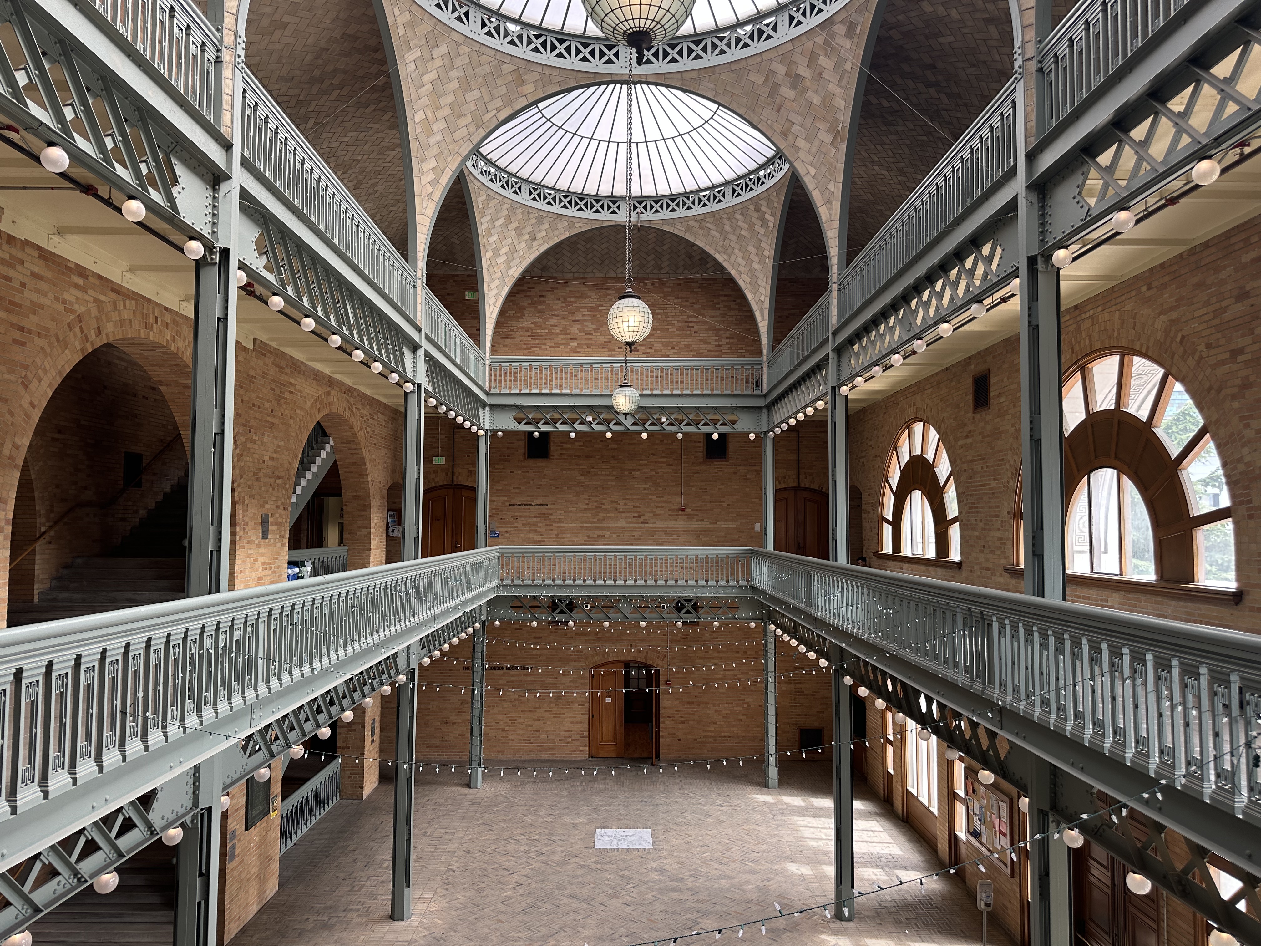
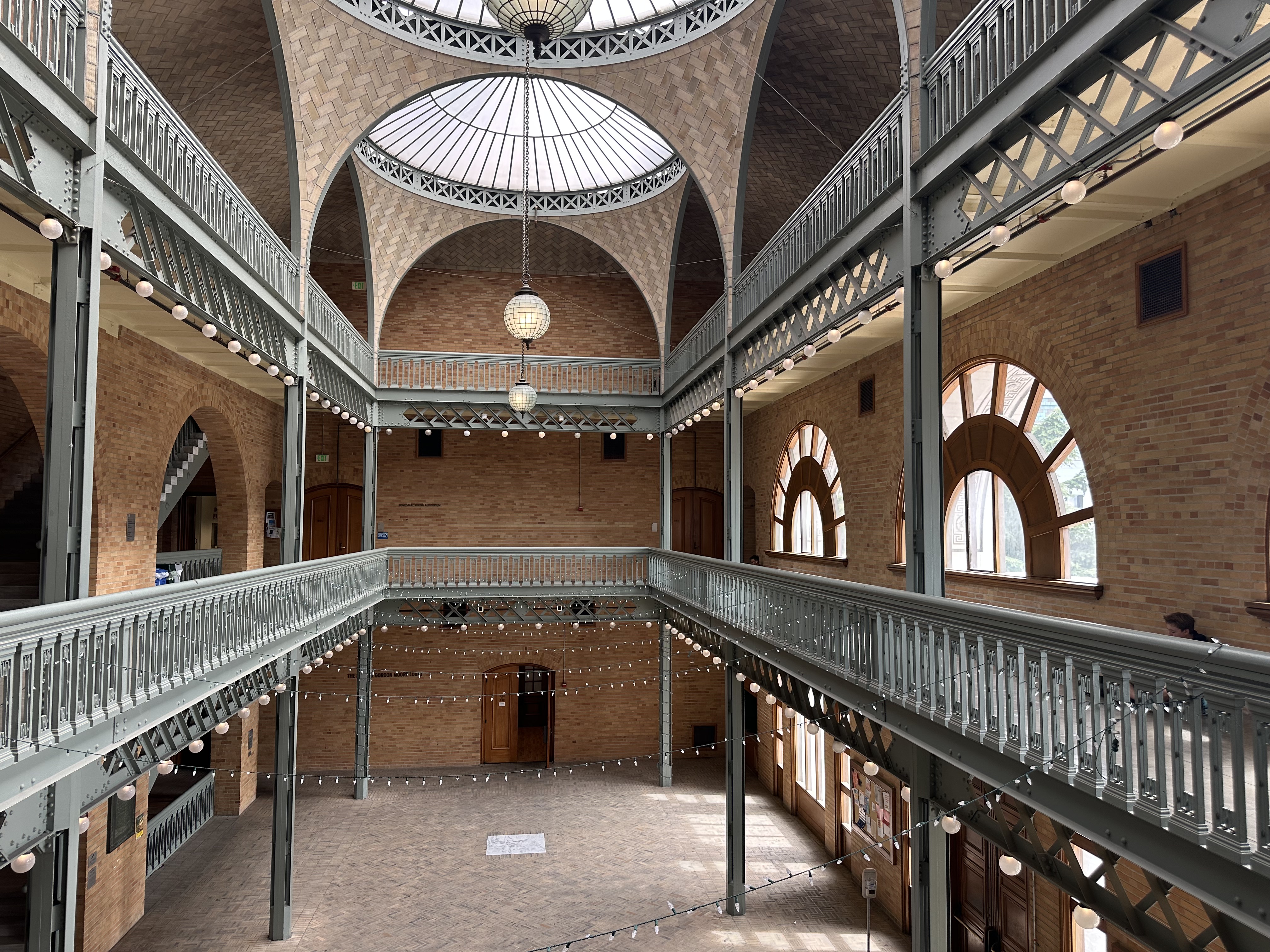
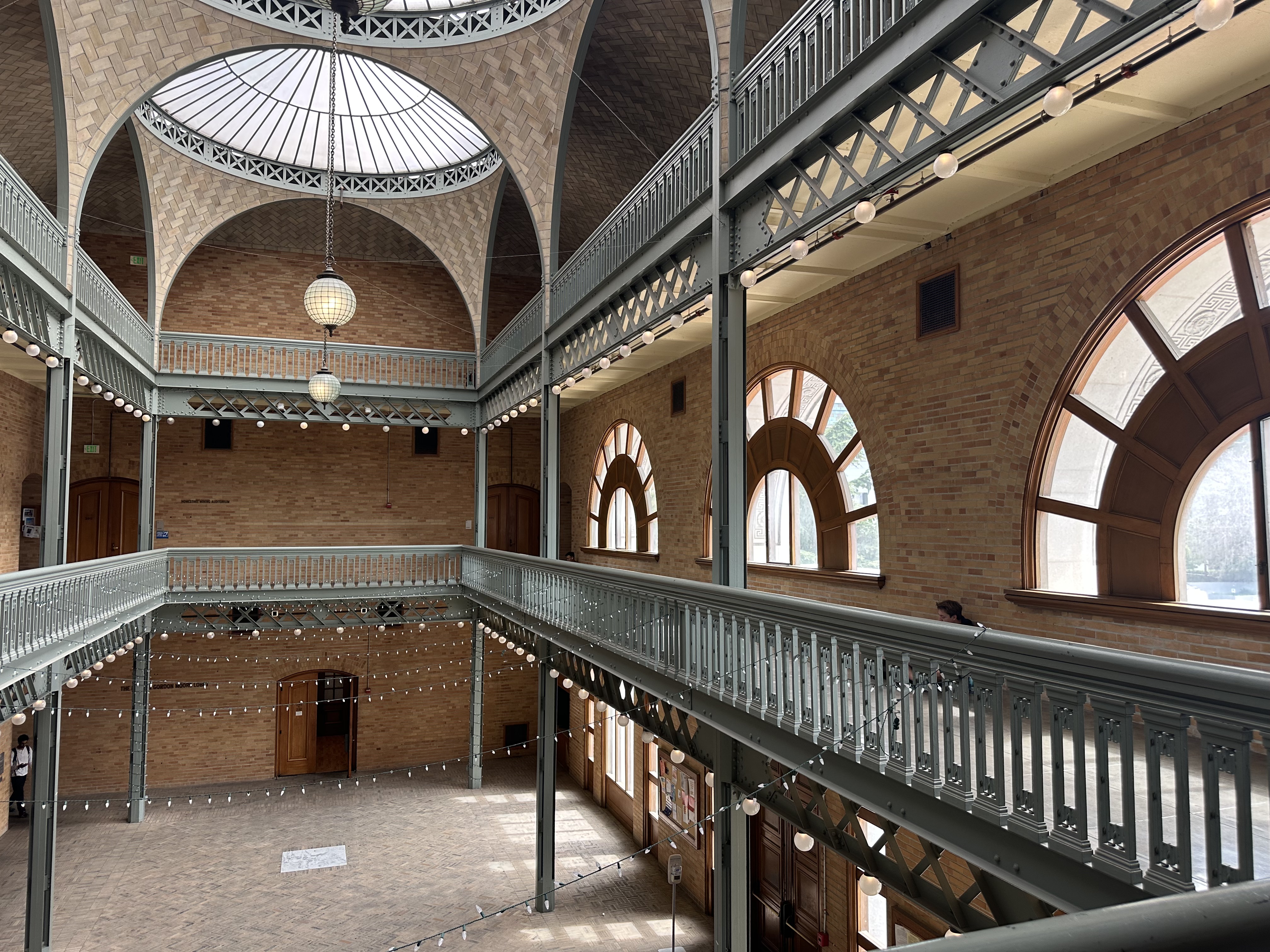
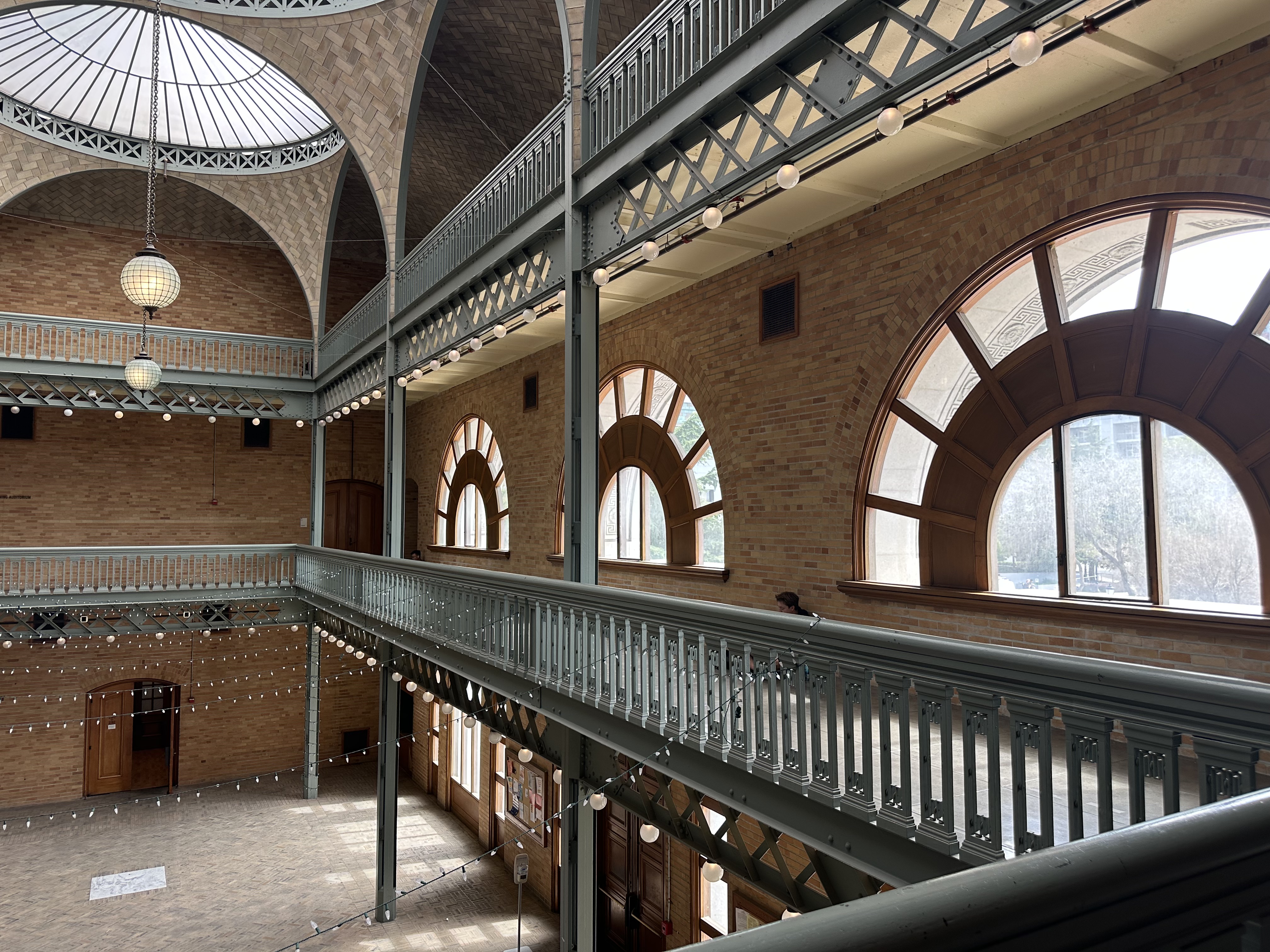
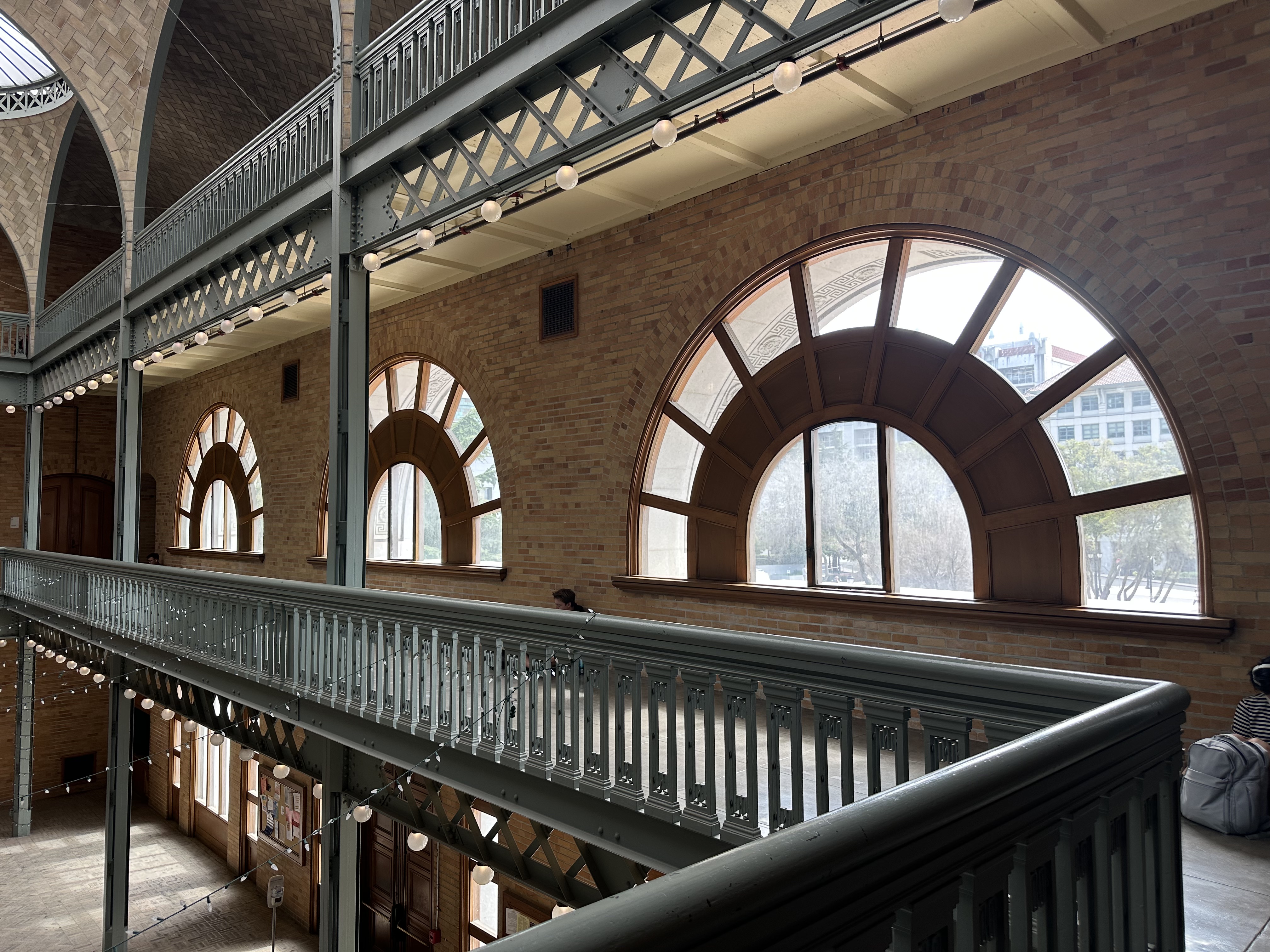
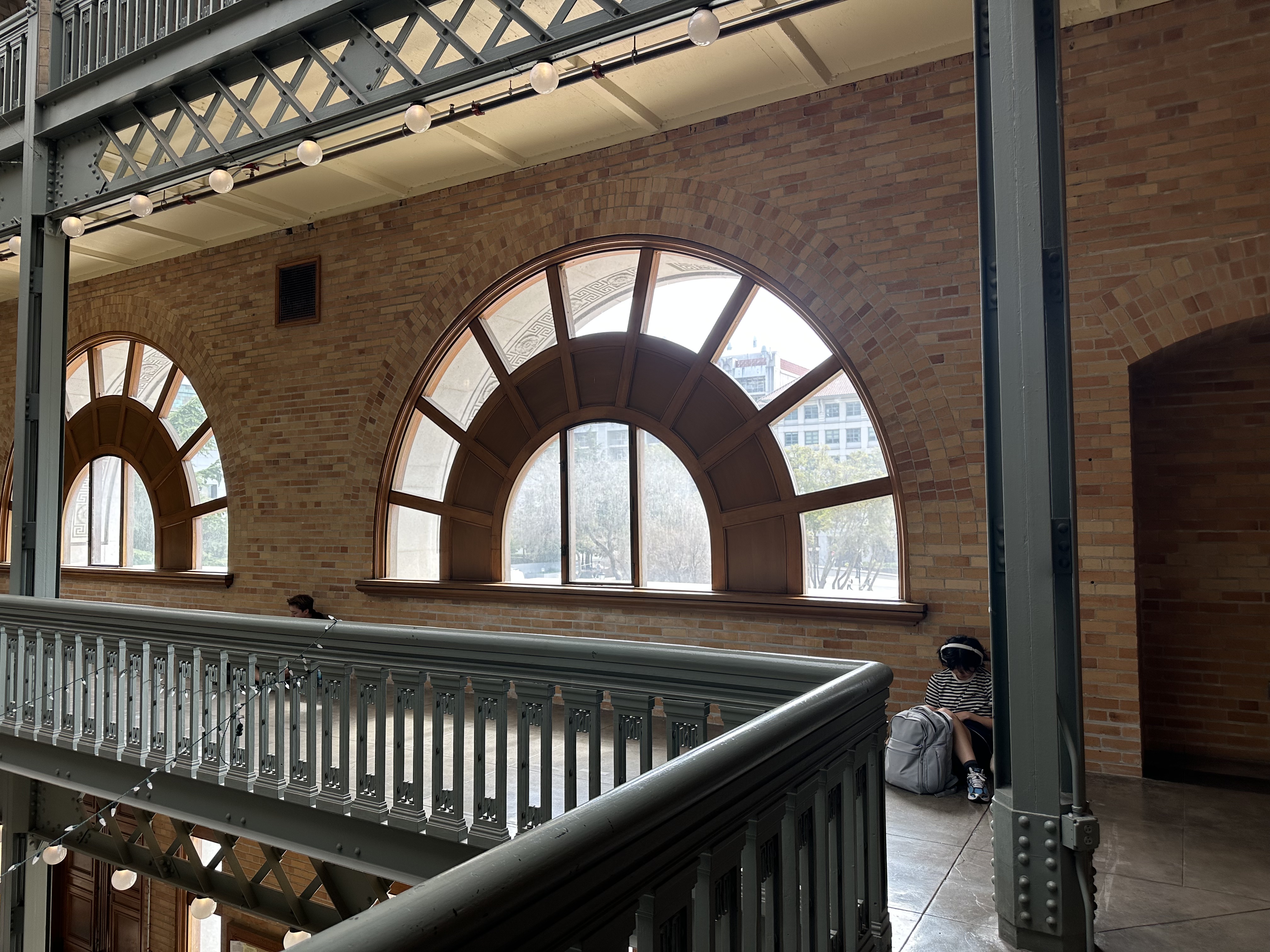
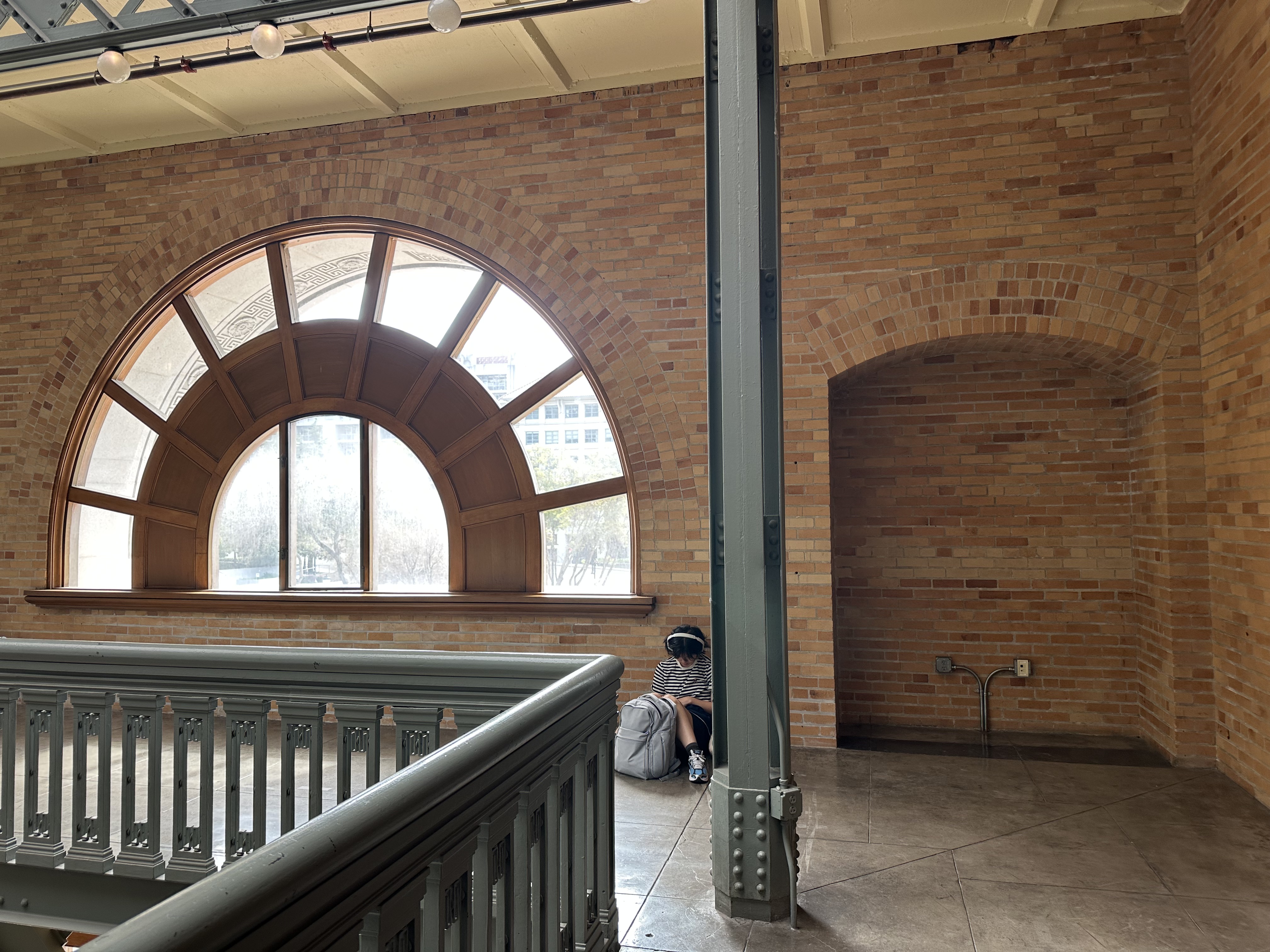
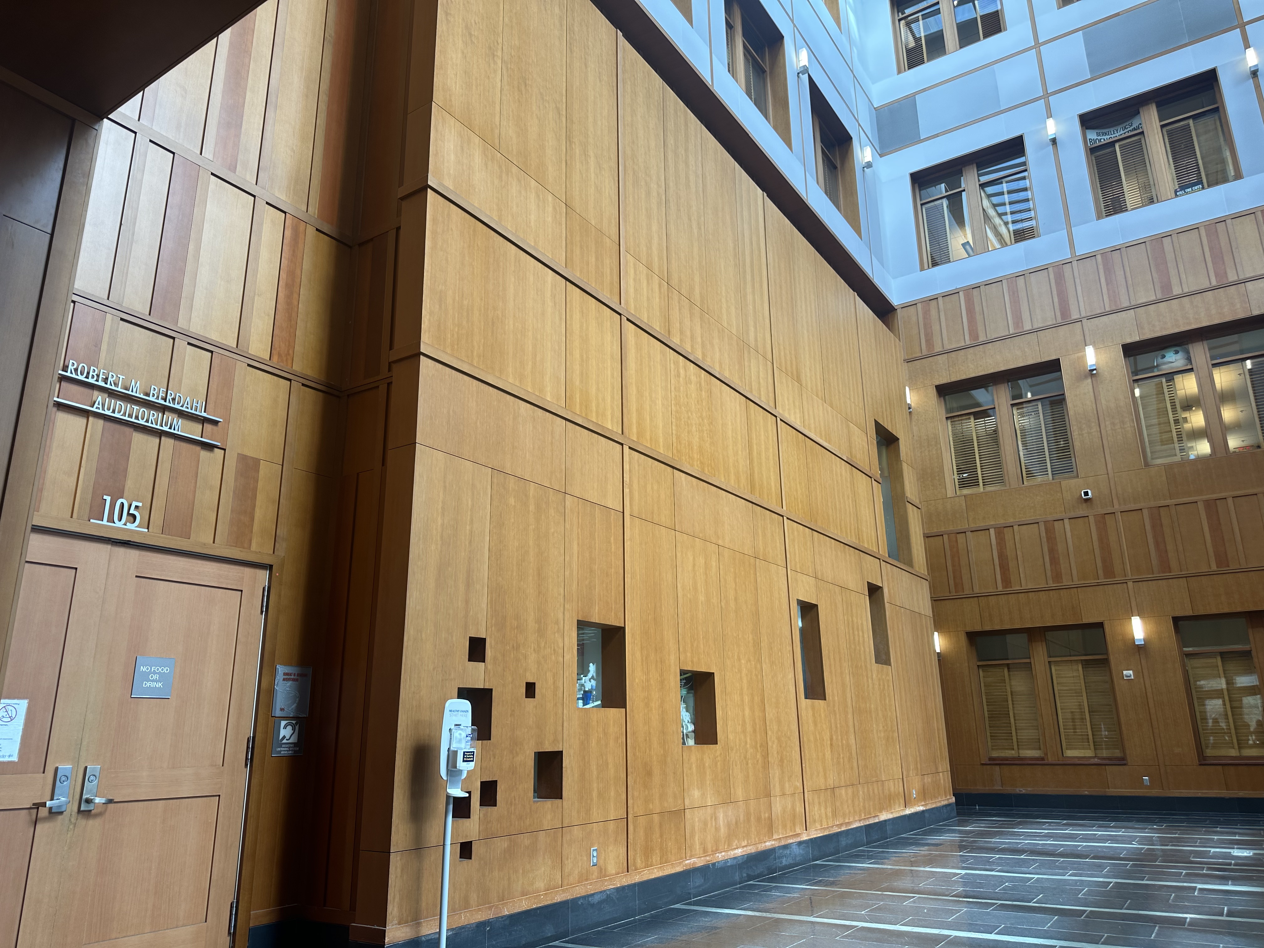
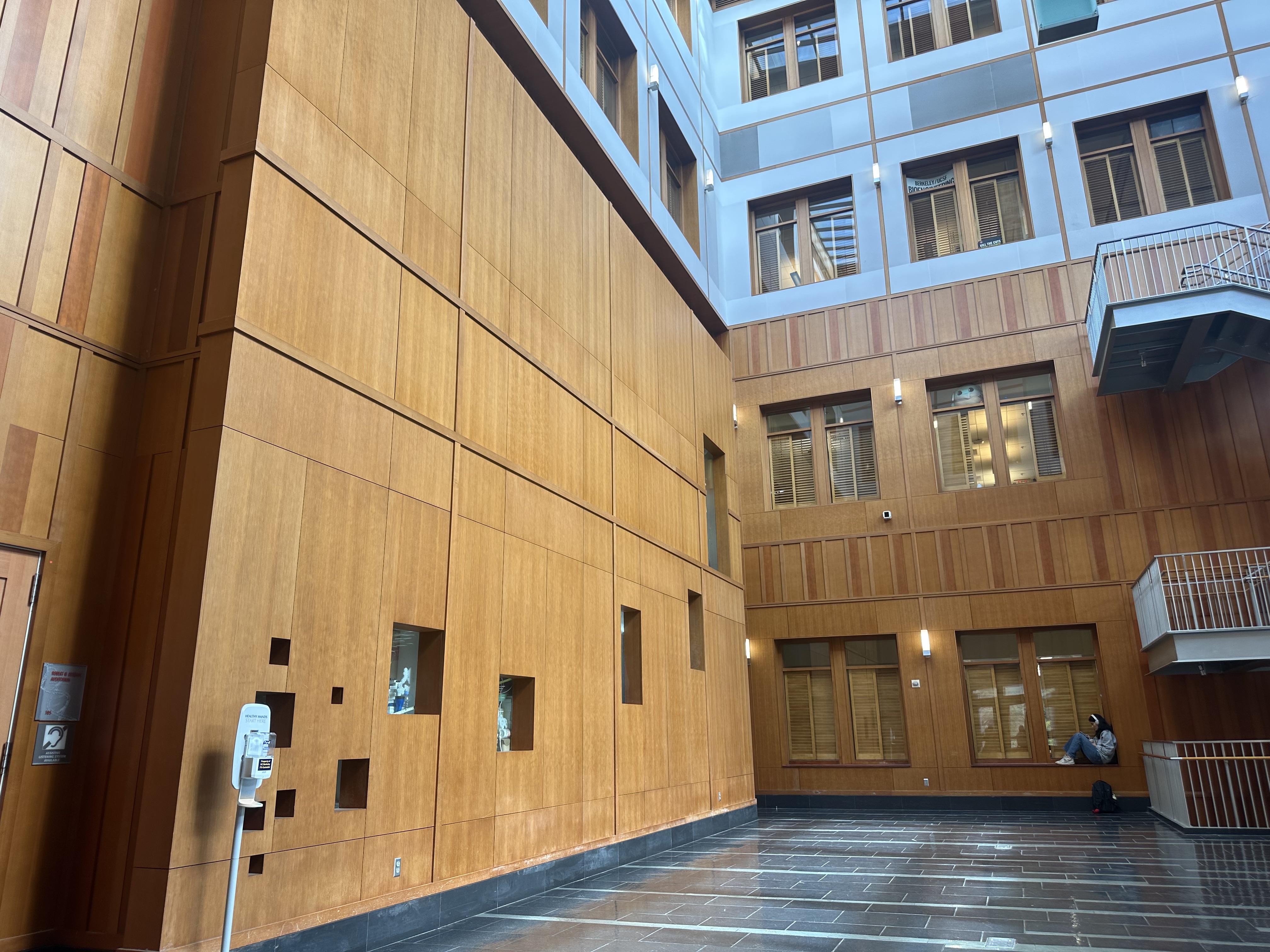
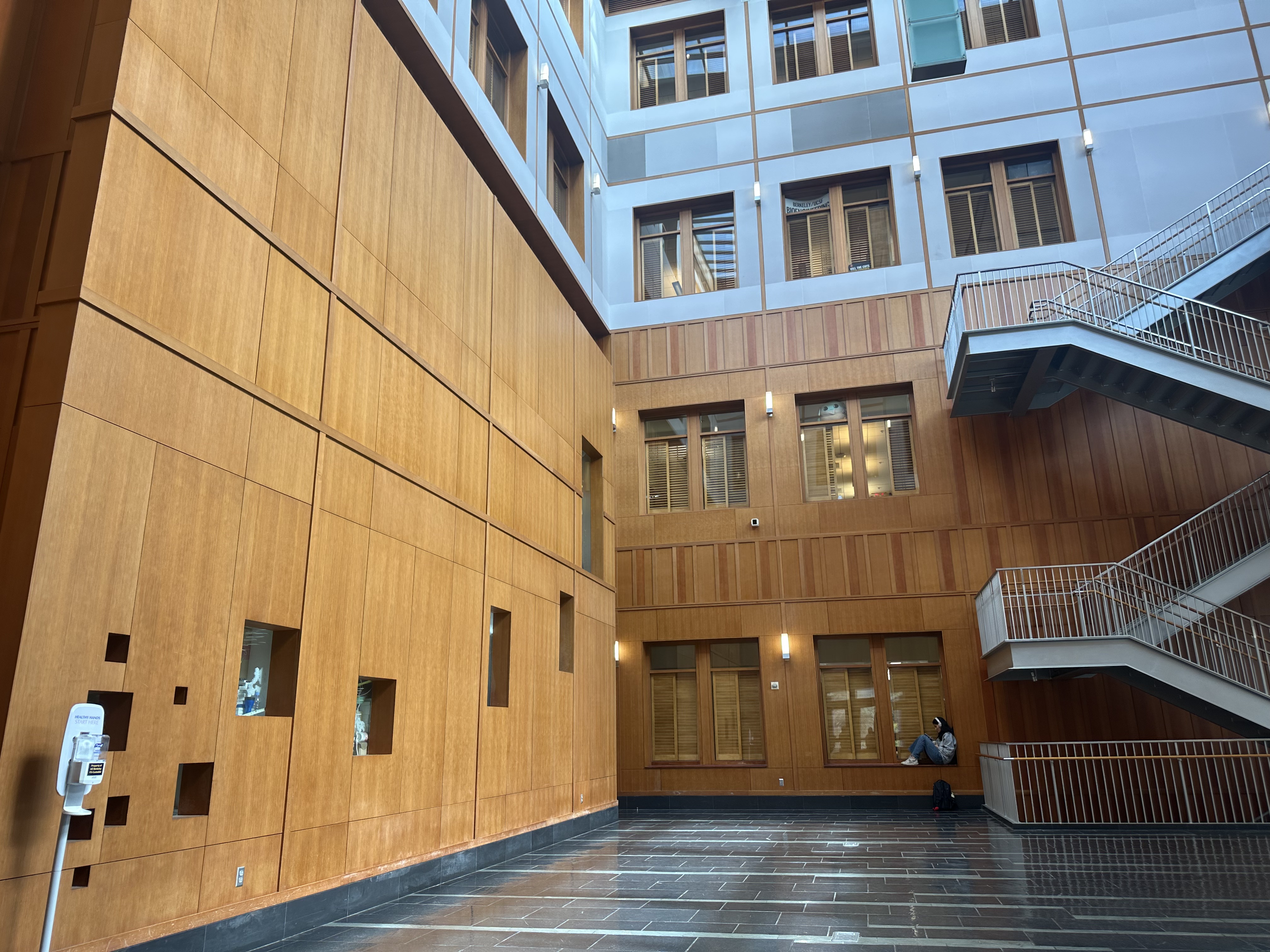
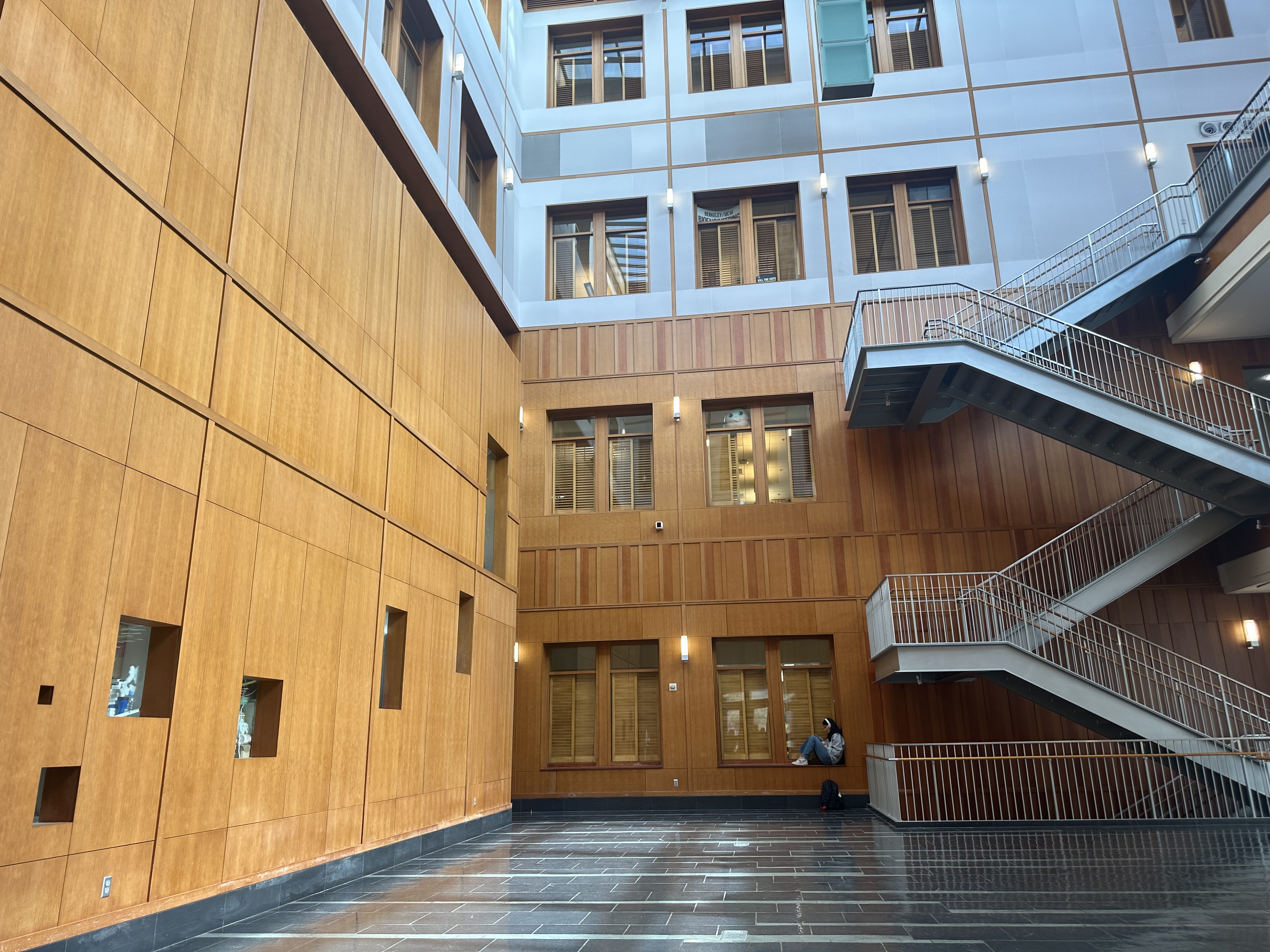
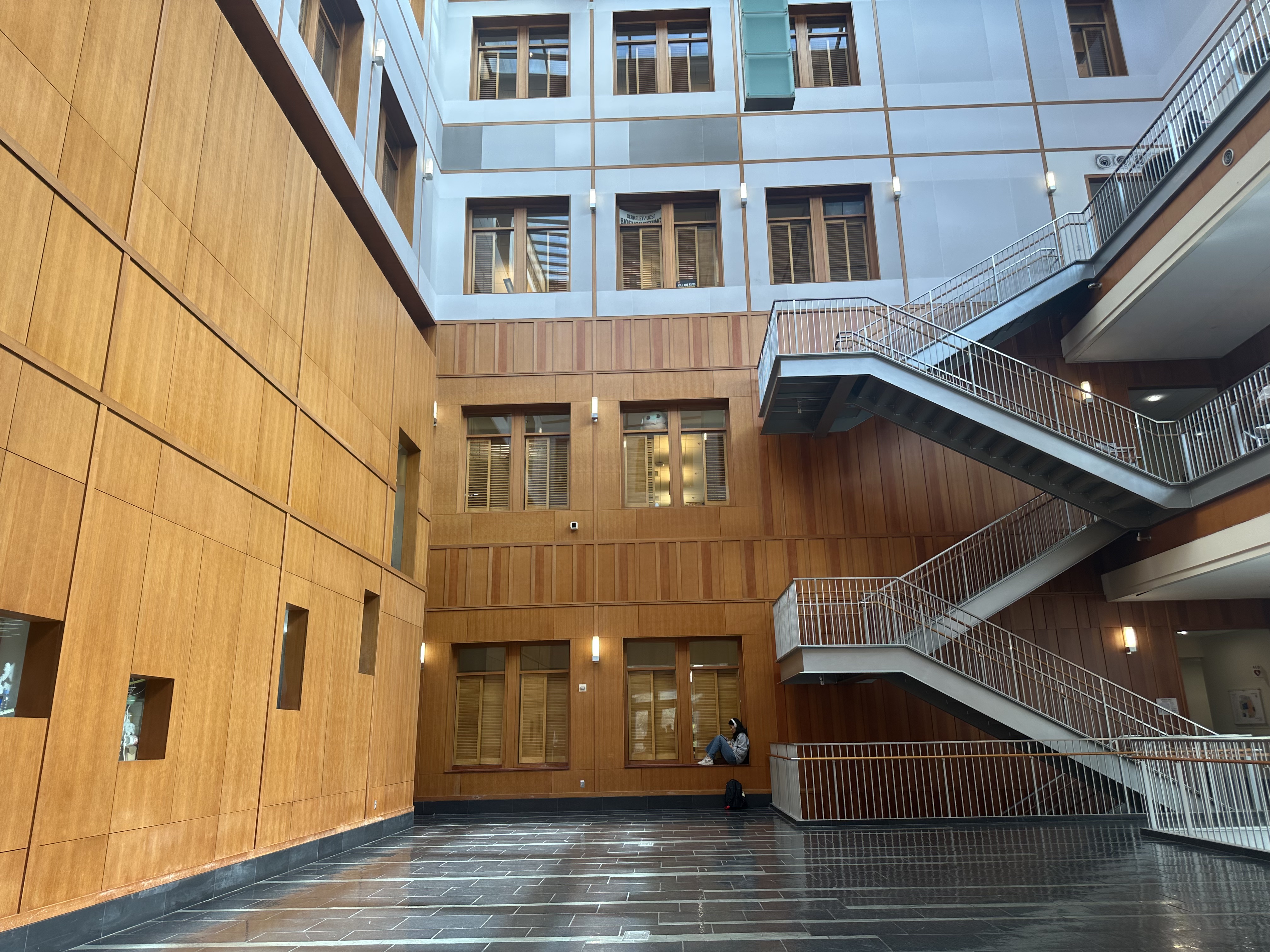
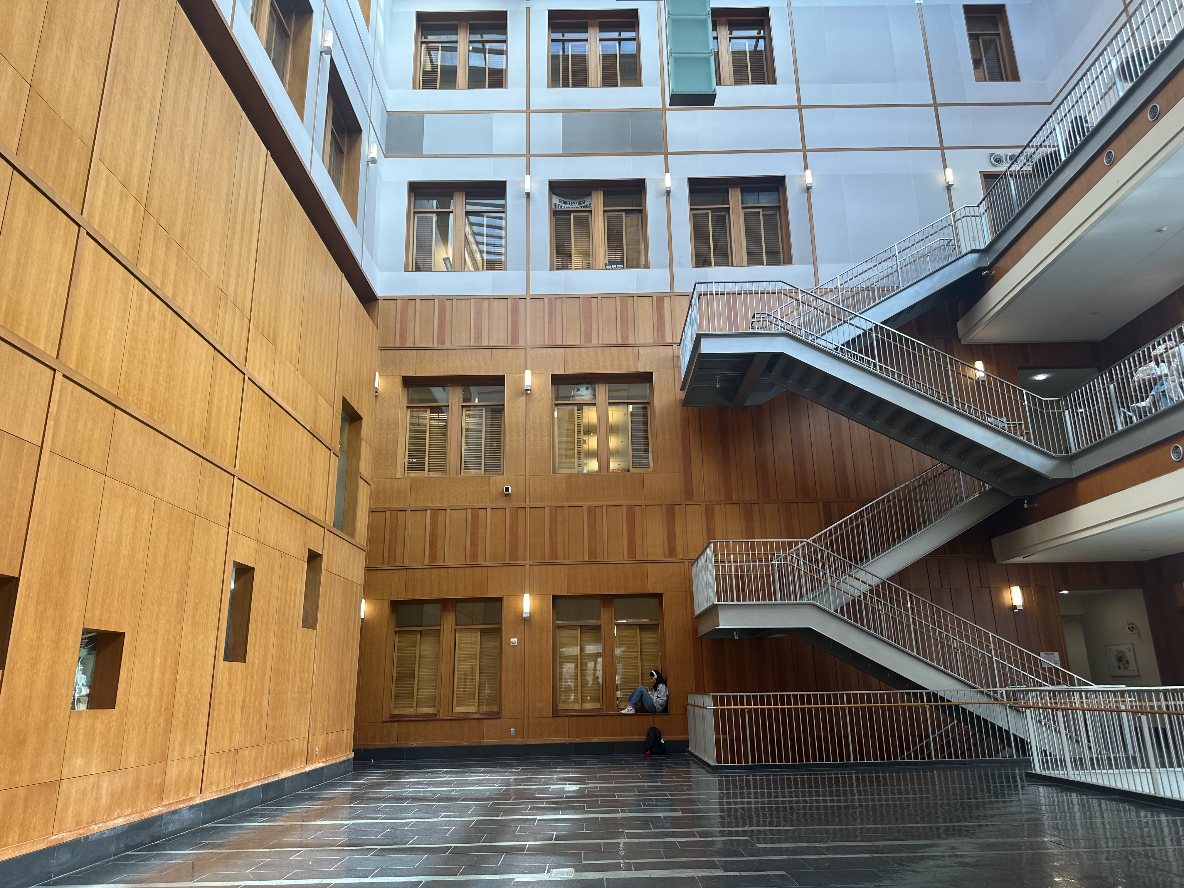
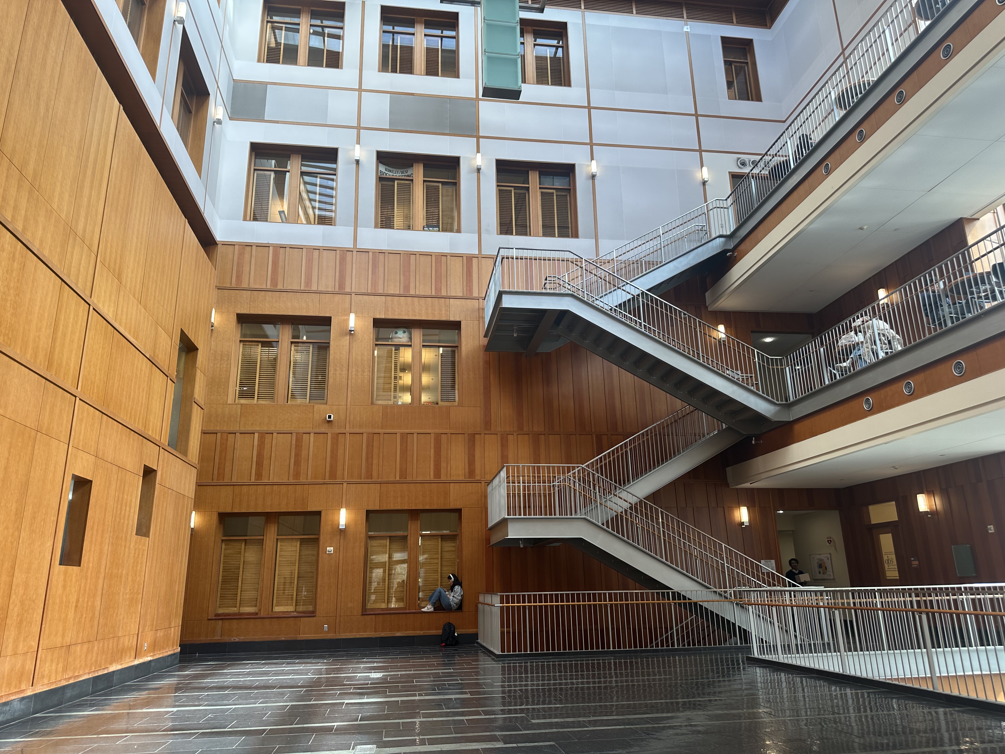
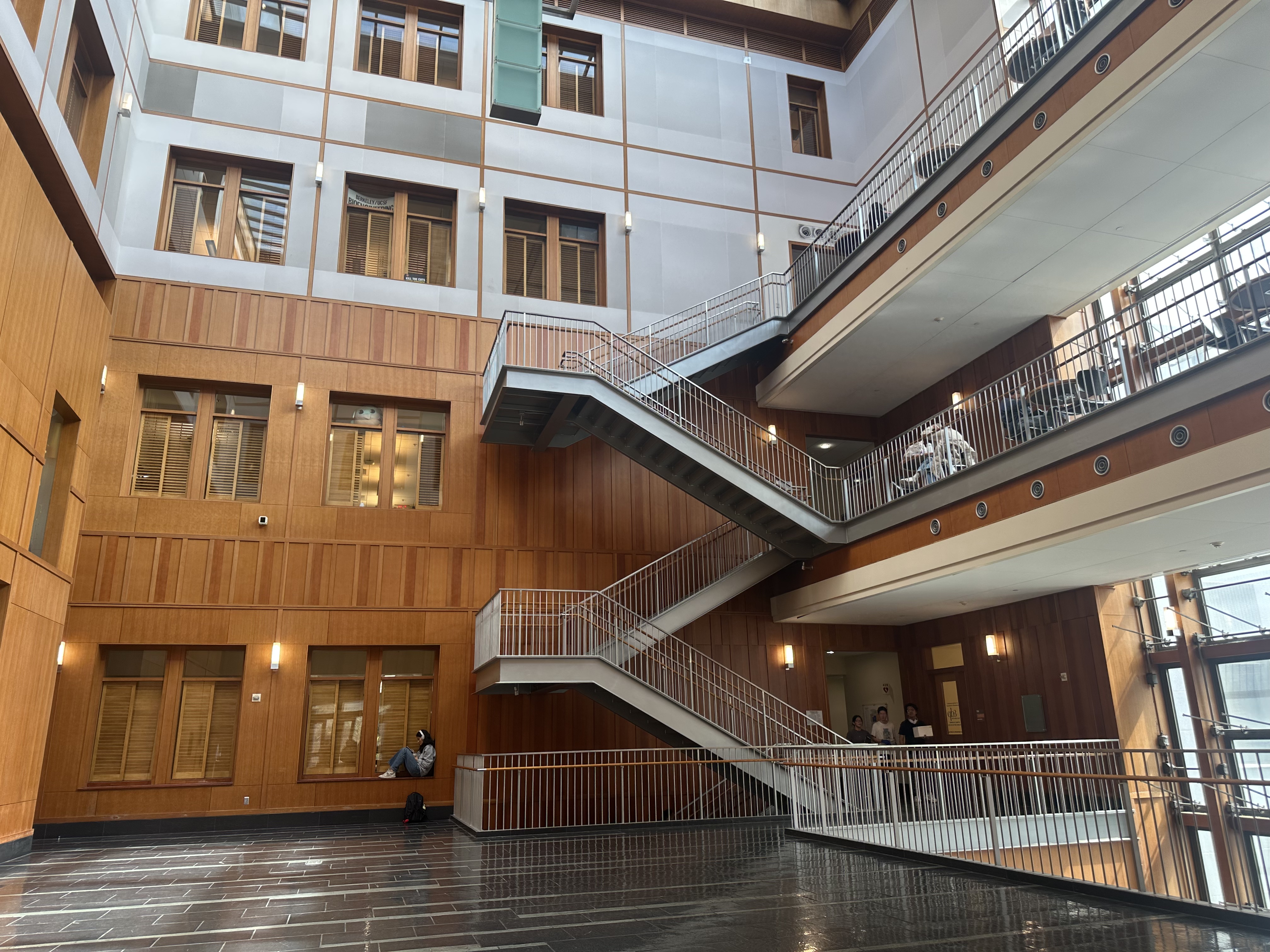
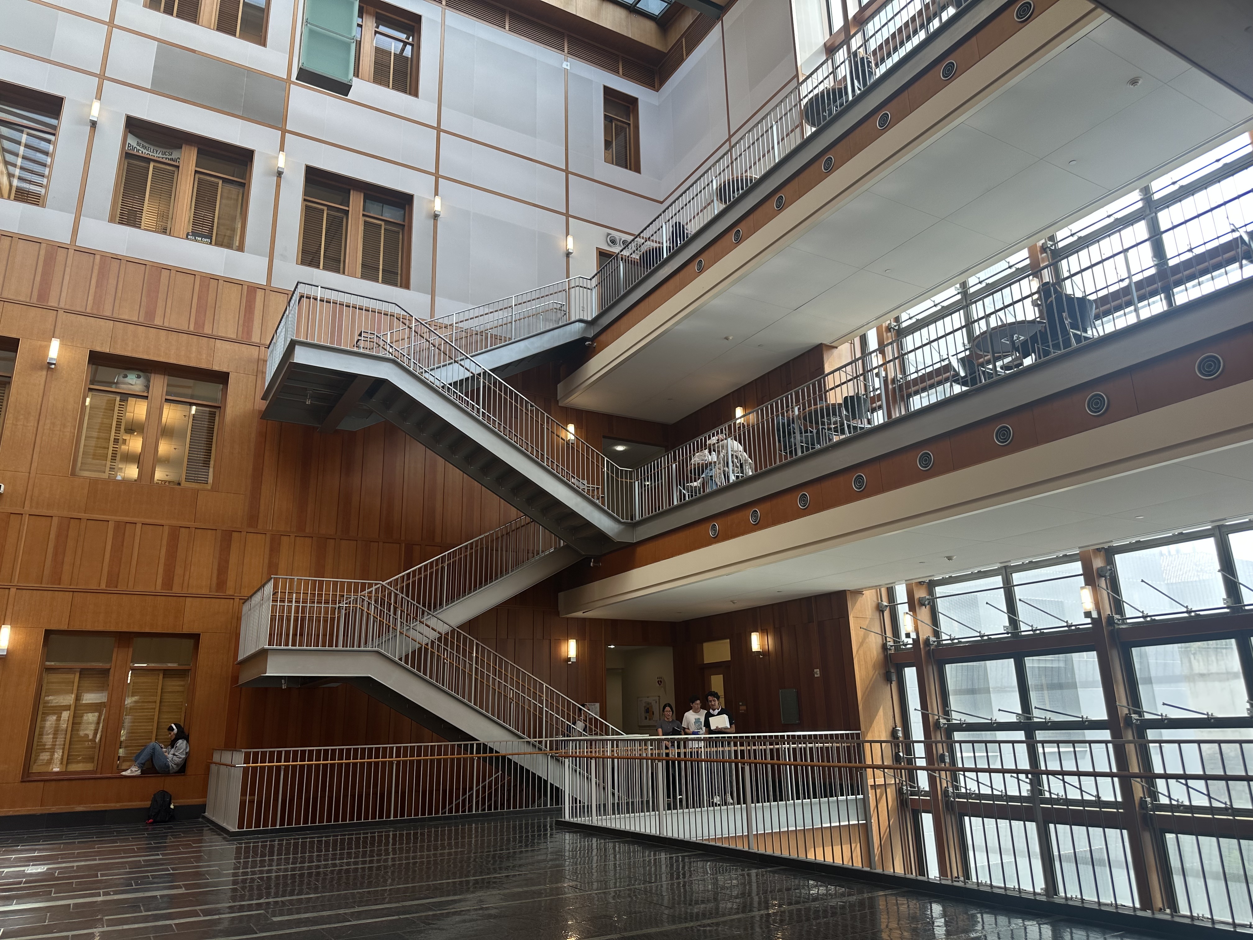
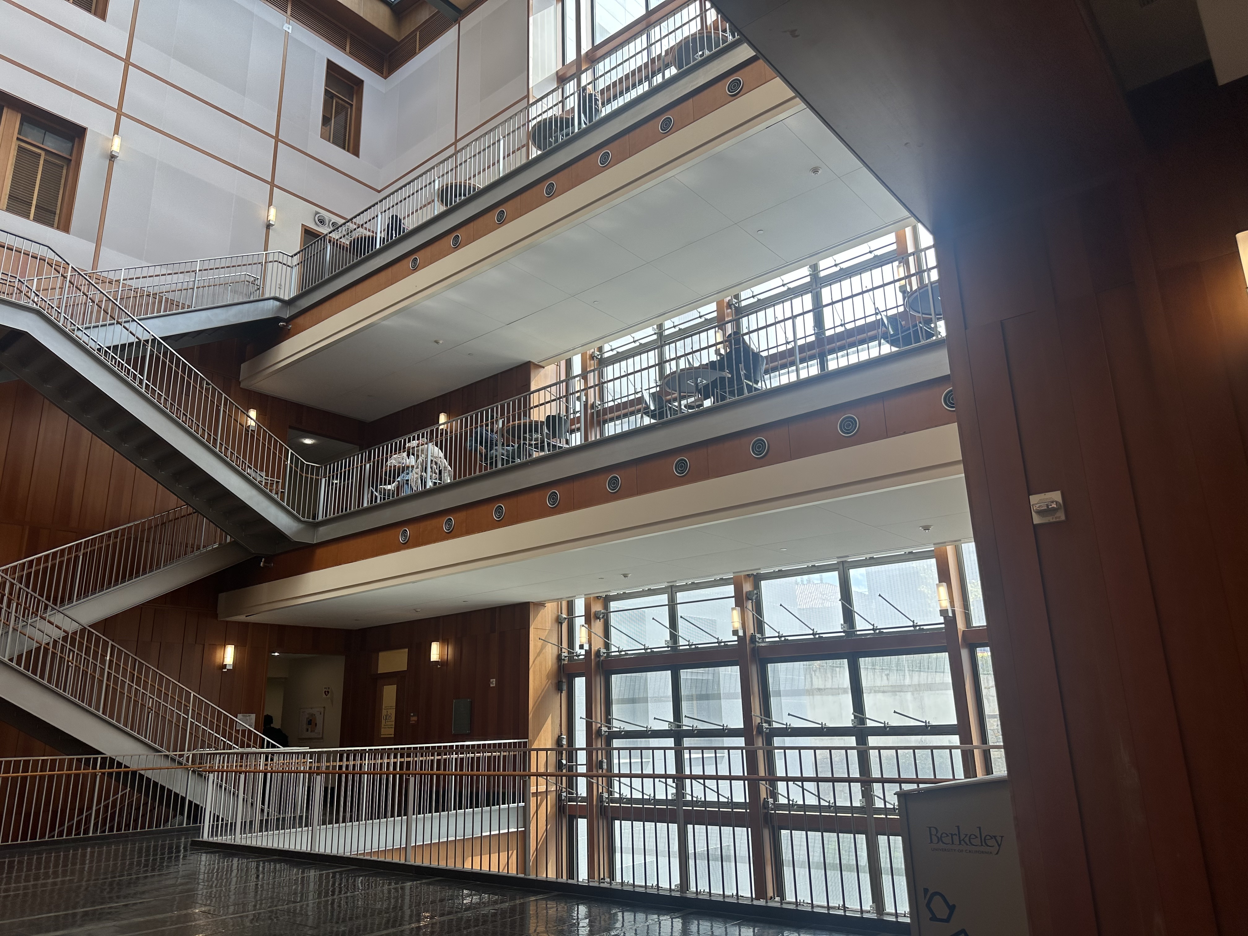
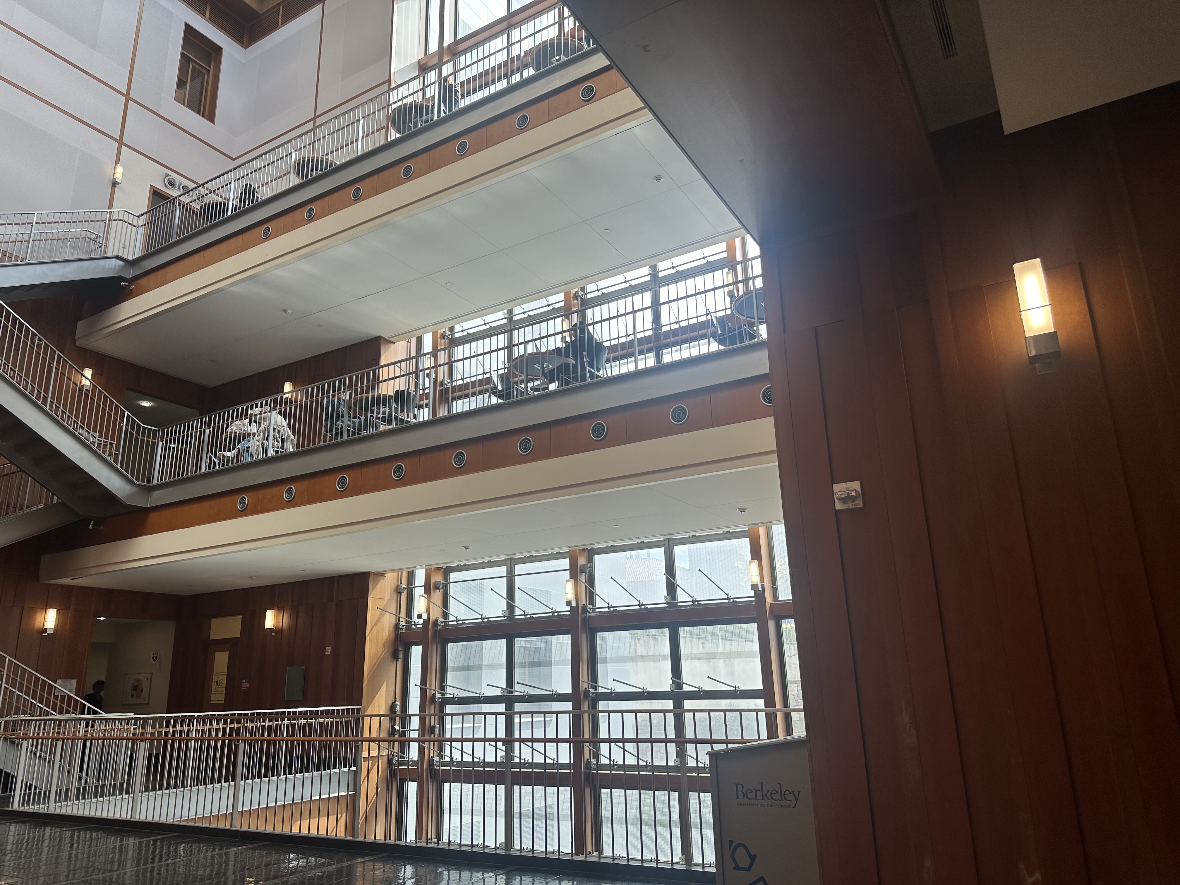
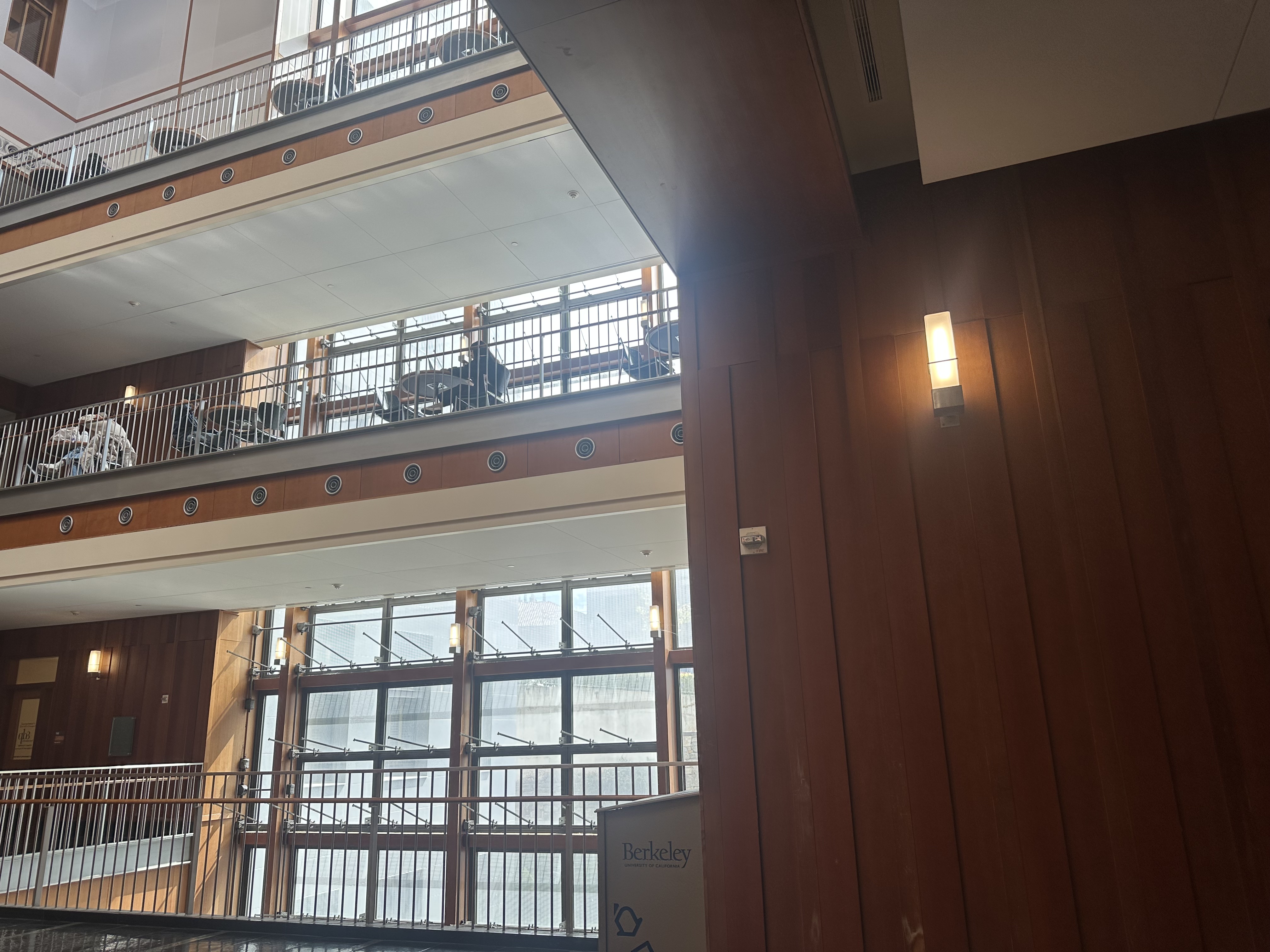
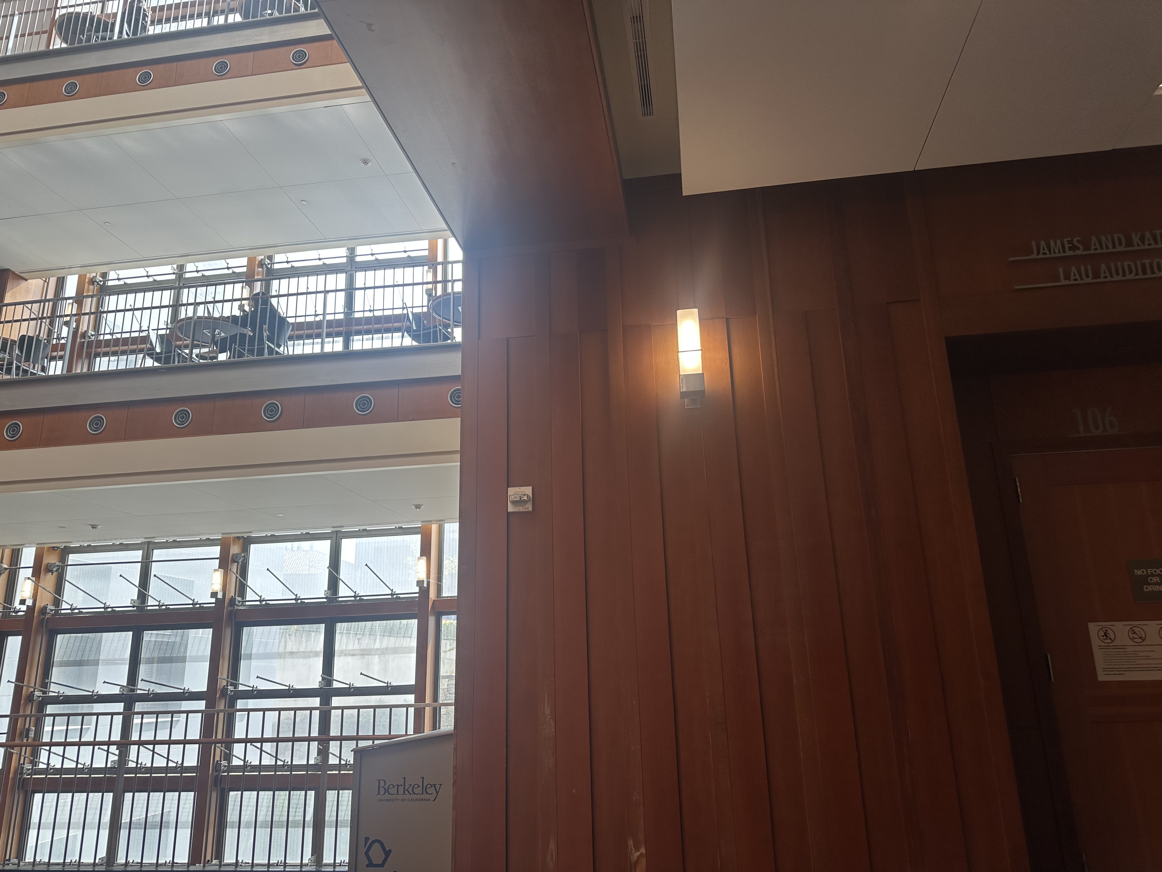
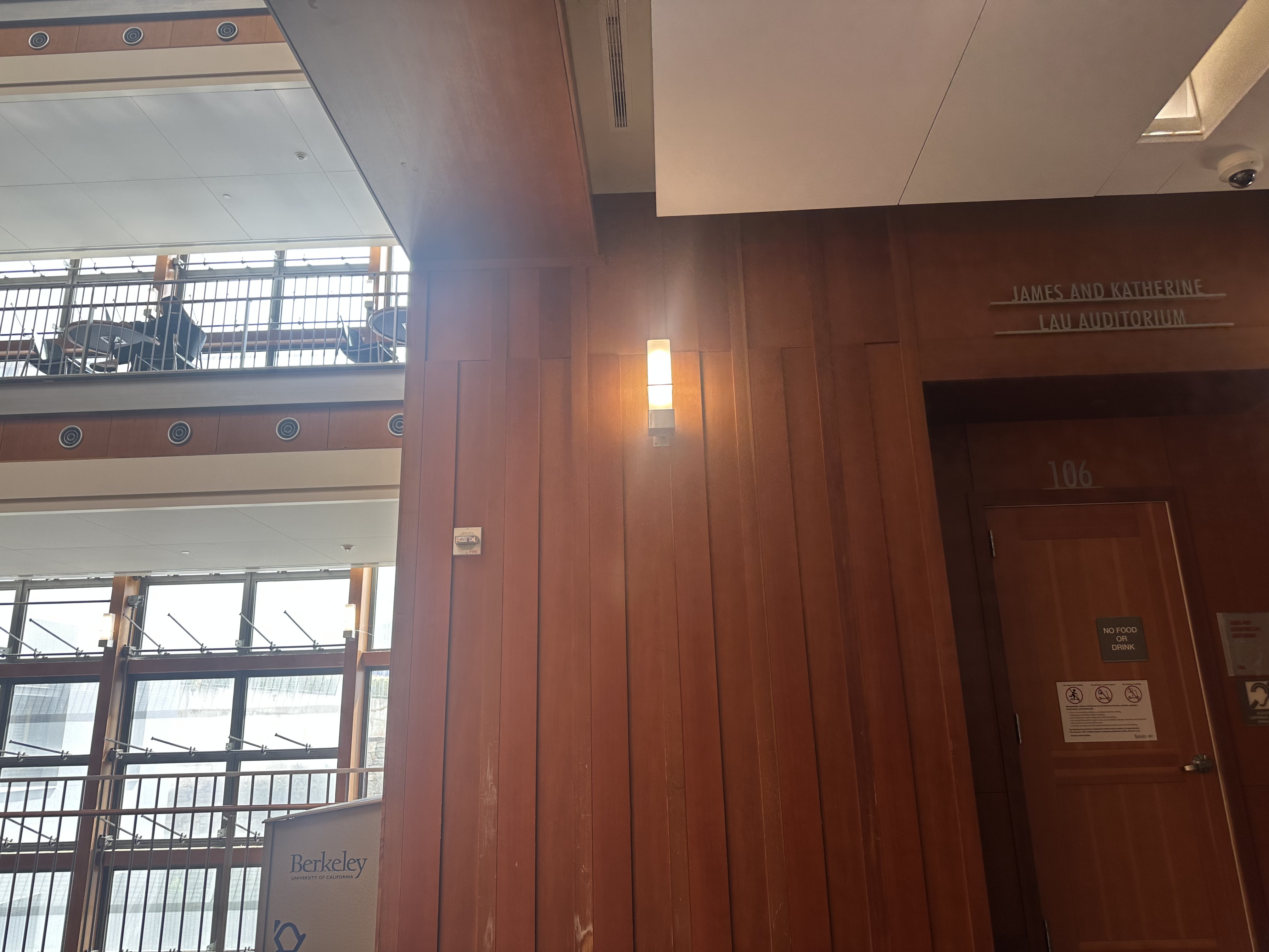
I captured multiple image sets with overlapping fields of view by rotating the camera around a fixed center of projection. This ensured projective transformations suitable for mosaic creation.

Set 1: Hearst Memorial Mining Building

Set 2: Stanley Hall

A.2: Recover Homographies

For homography recovery I manually picked N point pairs with ginput on the two images, im1_pts to im2_pts. From each correspondence (xi, yi) to (xi, yi), I added two rows to a design matrix A, with DLT constraints. In my code, I put the (y′) row first and the (x′) row second:

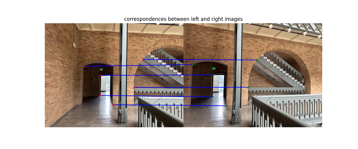
After stacking all pairs, I solve A h = 0 with SVD (U, S, Vt = np.linalg.svd(A)), take the last row of Vt, reshape to H, and normalize so that H[2,2] = 1. I also visualize the clicked correspondences by concatenating the two images side-by-side and drawing lines between matched points.

Visualized Correspondences:

System of equations for one match \((x,y)\to (u,v)\):

[-x -y -1  0  0  0  u x  u y  u]  ·  h = 0
[ 0  0  0 -x -y -1  v x  v y  v]  ·  h = 0
  

Recovered Homography Matrix (after SVD)

[[ 1.65836595e+00 -4.19105771e-03 -1.59991304e+03]
  [ 2.49401454e-01  1.42011820e+00 -6.34876480e+02]
  [ 1.56979836e-04  1.36539039e-05  1.00000000e+00]]

Below are the prints from my code: the Ah = 0 design matrix \(A\) and the first two rows corresponding to one correspondence pair.

Output of Ah=0 system:

[[ 0.00000000e+00  0.00000000e+00  0.00000000e+00 -1.64239622e+03
    -1.51502580e+03 -1.00000000e+00  2.47491285e+06  2.28297944e+06
     1.50689147e+03]
   [ 1.64239622e+03  1.51502580e+03  1.00000000e+00  0.00000000e+00
     0.00000000e+00  0.00000000e+00 -1.43279874e+06 -1.32168293e+06
    -8.72383117e+02]
   [ 0.00000000e+00  0.00000000e+00  0.00000000e+00 -1.90490069e+03
    -1.52017294e+03 -1.00000000e+00  2.88956294e+06  2.30596557e+06
     1.51691002e+03]
   [ 1.90490069e+03  1.52017294e+03  1.00000000e+00  0.00000000e+00
     0.00000000e+00  0.00000000e+00 -2.24387583e+06 -1.79068617e+06
    -1.17794898e+03]
   [ 0.00000000e+00  0.00000000e+00  0.00000000e+00 -1.97696074e+03
    -2.37974640e+03 -1.00000000e+00  4.76163098e+06  5.73176489e+06
     2.40856122e+03]
   [ 1.97696074e+03  2.37974640e+03  1.00000000e+00  0.00000000e+00
     0.00000000e+00  0.00000000e+00 -2.45749974e+06 -2.95819034e+06
    -1.24306957e+03]
   [ 0.00000000e+00  0.00000000e+00  0.00000000e+00 -2.58947117e+03
    -2.38489354e+03 -1.00000000e+00  6.12015745e+06  5.63664279e+06
     2.36347774e+03]
   [ 2.58947117e+03  2.38489354e+03  1.00000000e+00  0.00000000e+00
     0.00000000e+00  0.00000000e+00 -4.82734355e+06 -4.44596589e+06
    -1.86421985e+03]
   [ 0.00000000e+00  0.00000000e+00  0.00000000e+00 -2.70270839e+03
    -1.28340421e+03 -1.00000000e+00  3.47698921e+06  1.65107808e+06
     1.28648330e+03]
   [ 2.70270839e+03  1.28340421e+03  1.00000000e+00  0.00000000e+00
     0.00000000e+00  0.00000000e+00 -5.40398519e+06 -2.56612861e+06
    -1.99947032e+03]
   [ 0.00000000e+00  0.00000000e+00  0.00000000e+00 -2.84682849e+03
    -1.05178262e+03 -1.00000000e+00  3.06345418e+06  1.13181664e+06
     1.07609369e+03]
   [ 2.84682849e+03  1.05178262e+03  1.00000000e+00  0.00000000e+00
     0.00000000e+00  0.00000000e+00 -6.06292338e+06 -2.23999354e+06
    -2.12971150e+03]]

A.3: Warp the Images

To warp an image, I implemented inverse warping using the recovered homography matrix \(H\). I looped over every pixel in the output image, mapped it back into the input image using \(H^{-1}\), and sampled the corresponding color value.

I implemented two interpolation methods:

• Nearest Neighbor: Rounds the back-projected coordinates \((x, y)\) to the nearest integer pixel in the input image. This method is fast but produces blocky edges.
• Bilinear Interpolation: Computes a weighted average of the four neighboring pixels that surround the fractional coordinates. This yields a smoother, more natural-looking result, but it takes longer to compute.

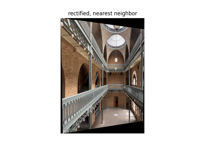
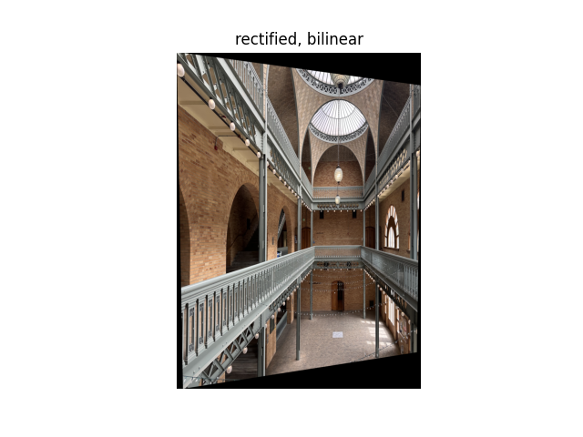
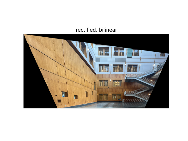
To rectify the image, I clicked four points and mapped them to a rectangle so they would be parallel.

Rectification Results & Comparison

A.4: Blend the Images into a Mosaic

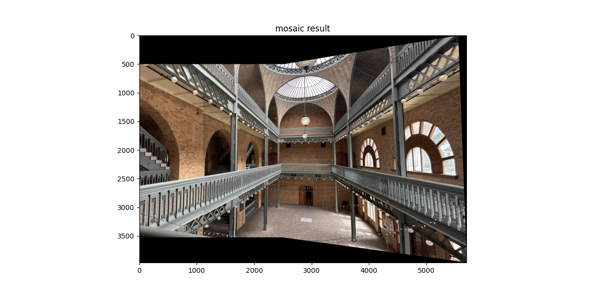
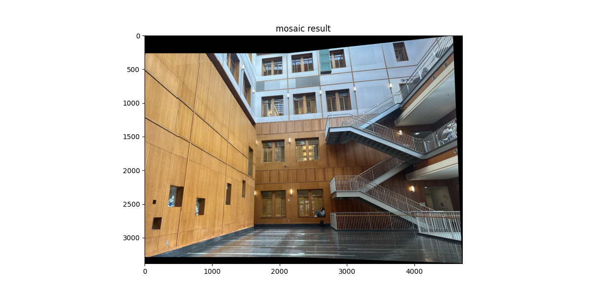
I implemented a simple image registration and blending process using homographies. After selecting correspondences between two overlapping images, I compute the homography H that maps points from the right image onto the left image’s frame. Then, I calculated the bounding box of the combined mosaic by transforming both images’ corners through H and determining their minimum and maximum extents. A translation matrix T shifts the coordinate system so that the final mosaic fits on a common canvas.

The right image is inverse-warped using bilinear interpolation (from A.3), while the left image is directly copied into the canvas. Overlapping regions are blended using a simple alpha weighting:

I_out = W_L * I_L + W_R * I_R

Here, W_L and W_R are normalized masks computed from the nonzero regions of each warped image. This weighted averaging smooths the seam between images and reduces ghosting artifacts. I also compared the results to a version without blending, where the right image only overwrites the left. The blended mosaics appear slightly more seamless near overlapping regions.

Mosaic 1

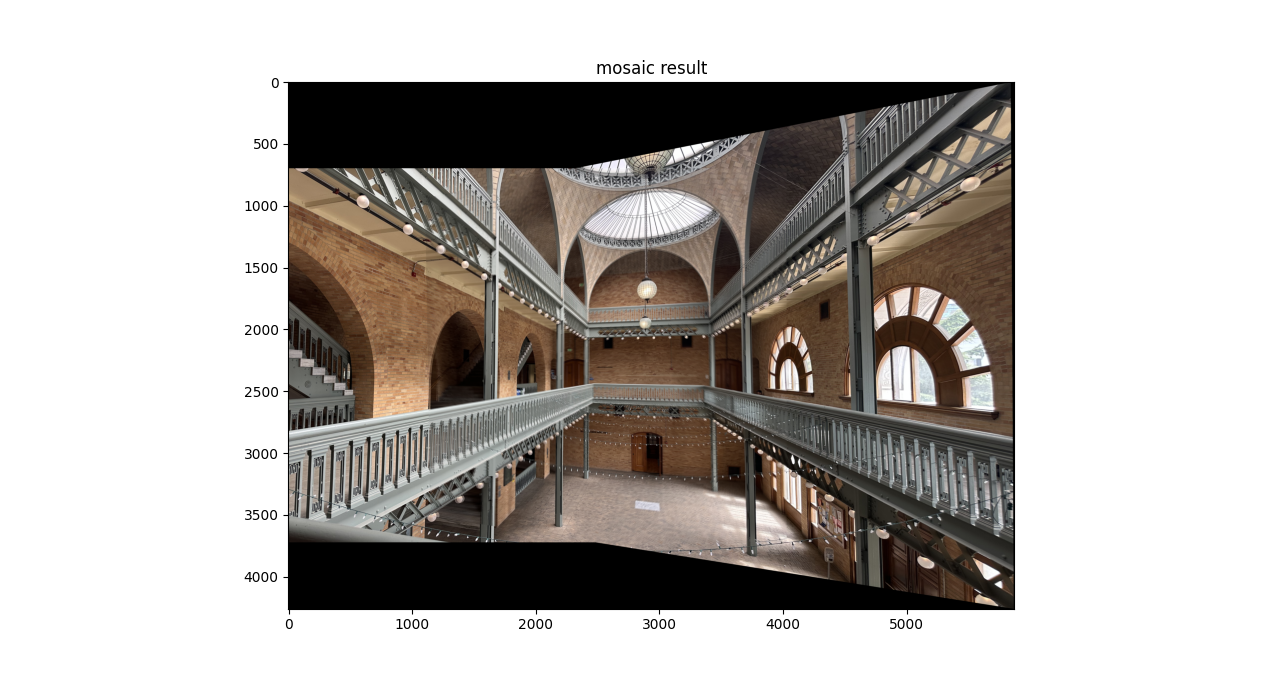Mosaic 2

Mosaic 3

Reference Paper for Part B

B.1: Harris Corner Detection

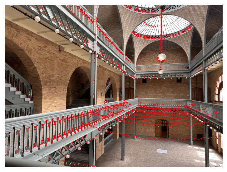
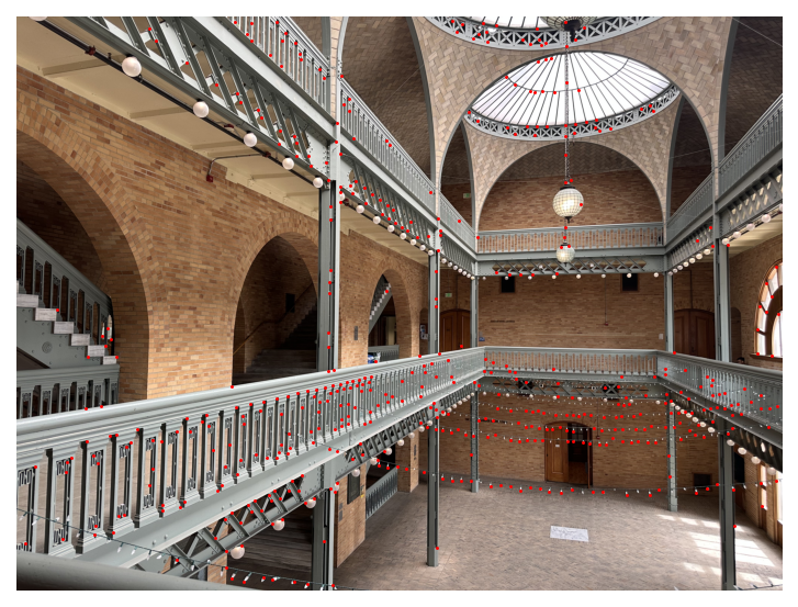
I ran the provided Harris detector then applied Adaptive Non-Maximal Suppression (ANMS) as in Section 3 of the paper.

Detected corners overlaid on the image, with and without ANMS:

B.2: Feature Descriptor Extraction

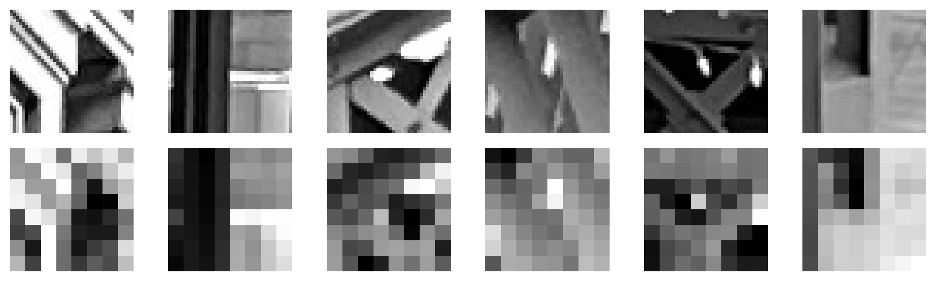
For each ANMS keypoint, I took a 40×40 grayscale window centered at the point, downsampled it to 8×8 by averaging non-overlapping 5×5 blocks, then bias/gain-normalized.

Normalized 8x8 feature descriptors with their source windows:

B.3: Feature Matching

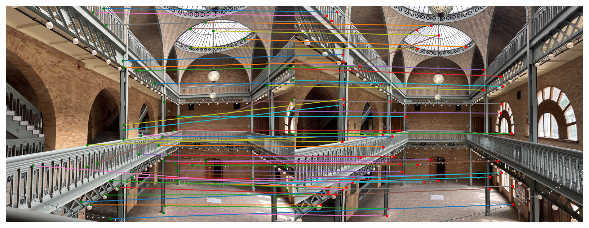
I matched descriptors using L2/SSD distances. For each descriptor in Image 1 I found the nearest and second-nearest in Image 2 and applied the Lowe ratio test (best/second < τ).

Matched features between image pairs:

B.4: RANSAC for Robust Homography

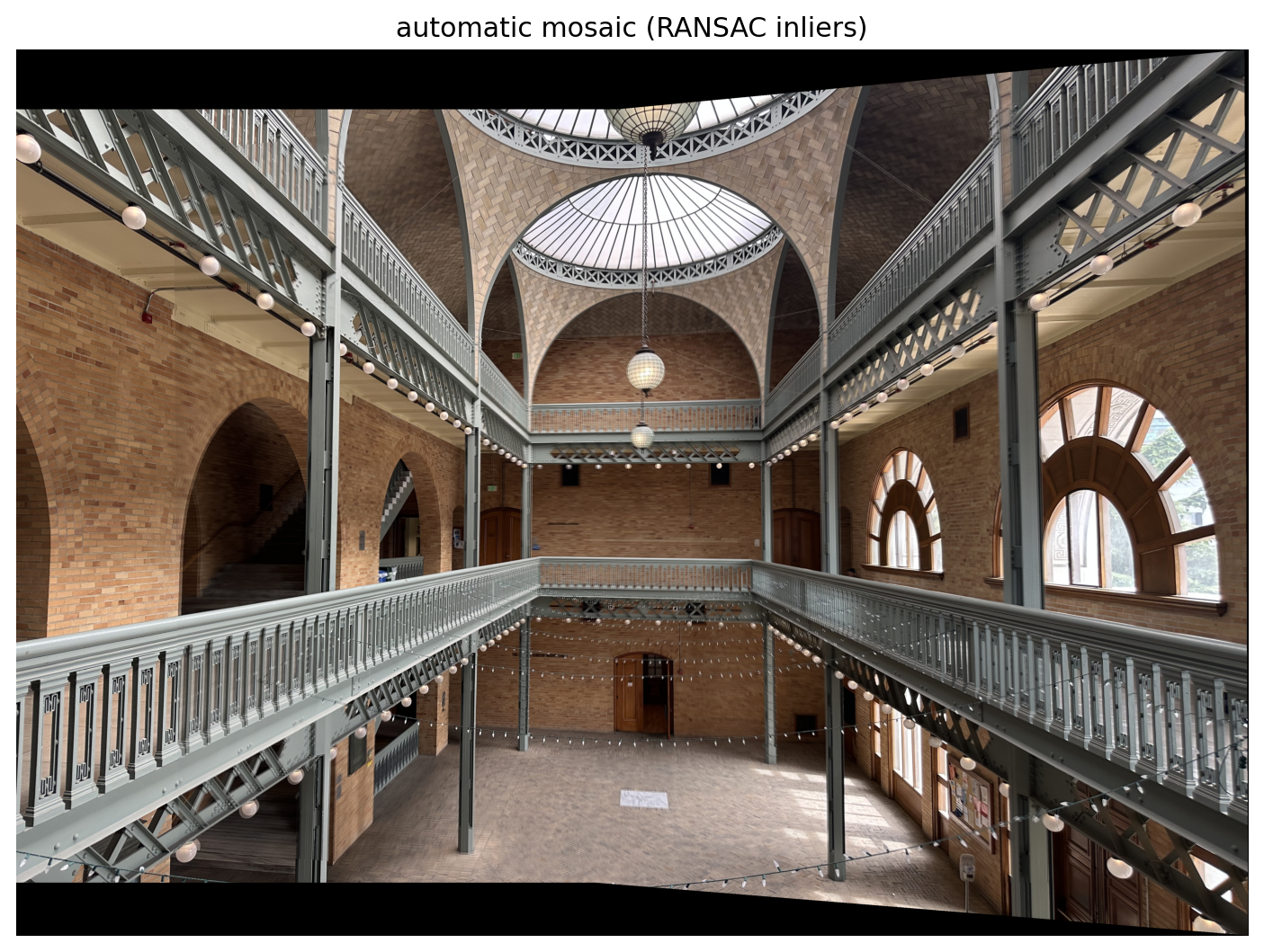
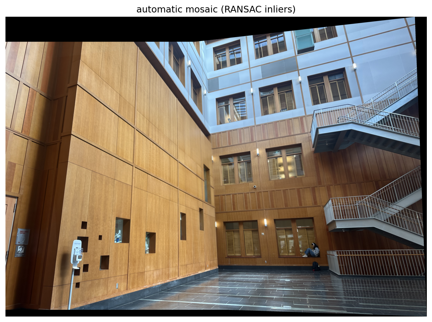
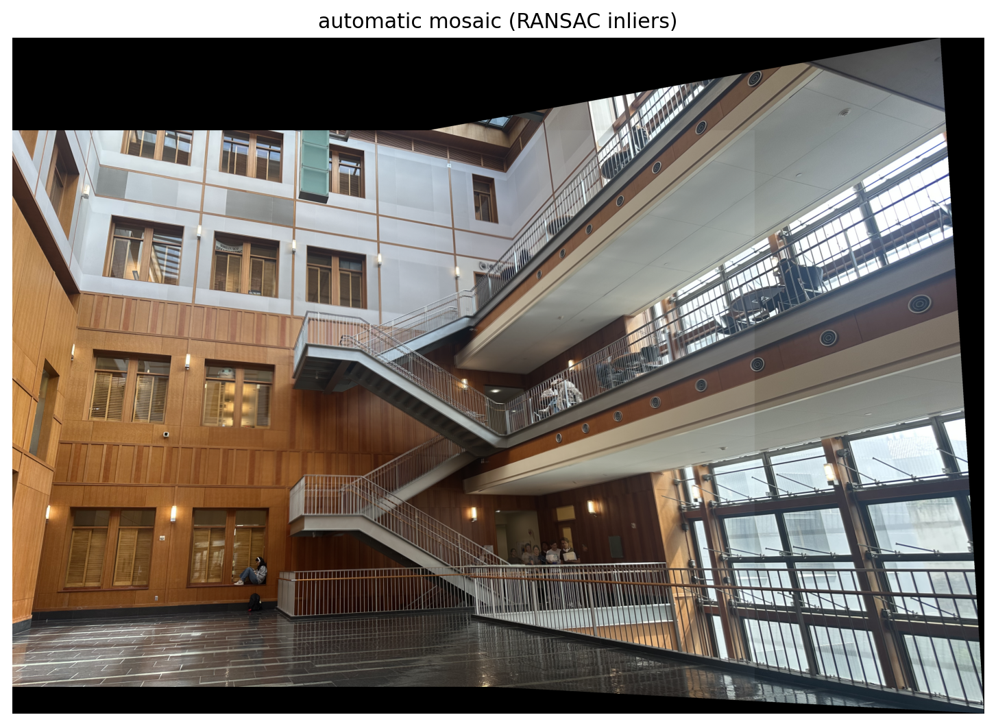
I implemented 4-point RANSAC following the loop taught in class: first, select four feature pairs at random. Second, compute exact homography with DLT. Then, count inliers using one-sided reprojection error, keep the largest set of inliers, and finally recompute least squares \(H\) estimate on all inliers.

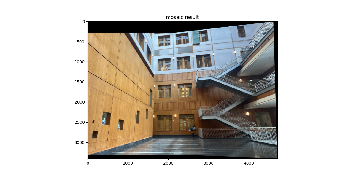
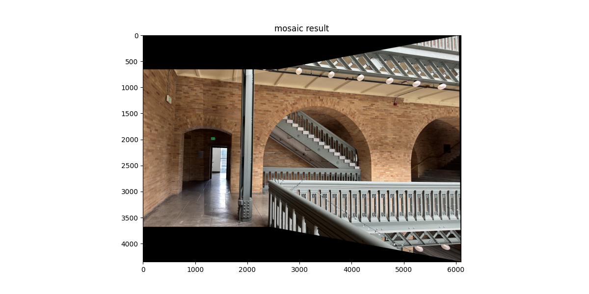
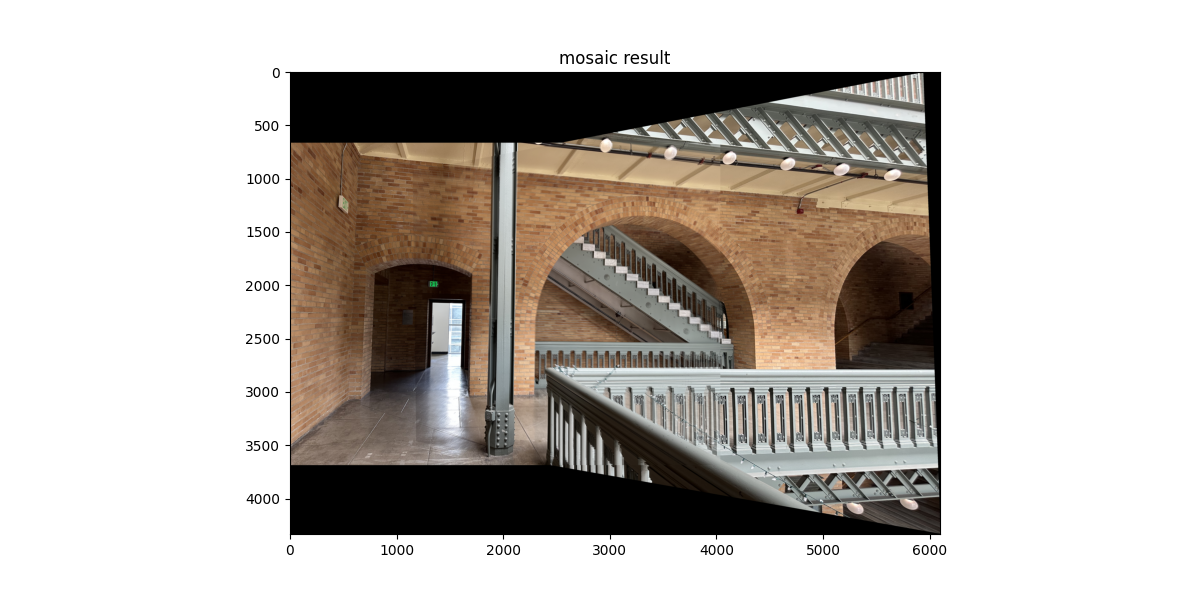
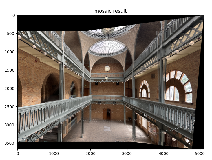
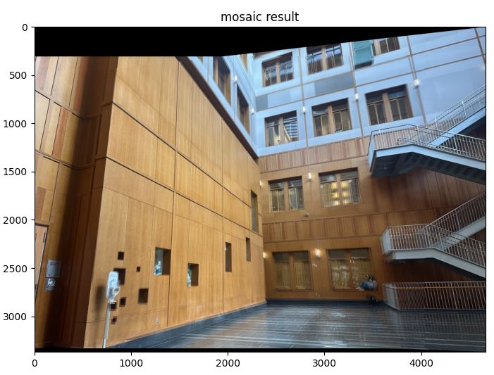
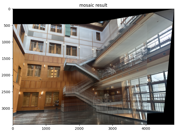
The manual mosaics were a lot shakier and unstable due to human error, my clicked correspondences weren't accurate/off by a few pixels. The small mistakes amplified in the homography, showing ghosting across the seams. RANSAC discards outliers automatically, so the automatic warps and steadier.

Manual vs. Automatic

Reflecting on the project, it really made me appreciate the entire pipeline. When Harris gives us too many points, ANMS makes them usable and the normalized descriptors and Lowe ratio play an integral role. I learned how sensitive homographies are, and I experienced a lot of difficulties clicking them exactly right, creating big seams. I appreciate how RANSAC helps avoid mistakes like that. Overall, the project helped improve my geometric intuition!